Appendix
This section covers some of the computational algorithms we use in CC3D
Calculating the Shape Constraint of a Cell – the Elongation Term
Calculating center of mass when using periodic boundary conditions.
Calculating Inertia Tensor in CC3D
Related: Calculating the Shape Constraint of a Cell – the Elongation Term and MomentOfInertia Plugin
- Learning Objectives:
Learn how CC3D calculates diagonal and off-diagonal inertia tensors
Prerequisite: Wikipedia: What is a Moment of Inertia?
For each cell, the inertia tensor is defined as follows:
where index \(i\) denotes i-th pixel of a given cell and \(x_i\),
\(y_i\) and \(z_i\) are coordinates of that pixel in a given
coordinate frame.
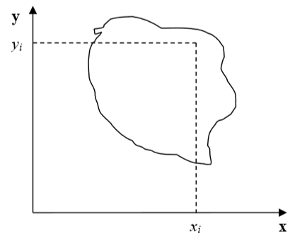
Figure 3: Cell and coordinate system passing through the center of mass of a cell. Notice that as the cell changes shape, the position of the center of mass moves.
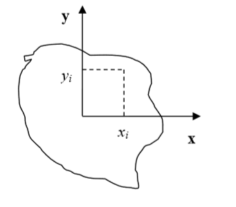
Figure 4: Cell and its coordinate frame in which we calculate inertia tensor
In Figure 4, we show one possible coordinate frame in which one can calculate the inertia tensor. If the coordinate frame is fixed calculating components of inertia tensor for cell gaining or losing one pixel is quite easy. We will be adding and subtracting terms like \(y_i^2+z_i^2\) or \(x_i z_i\).
However, in CompuCell3D, we are mostly interested in knowing the tensor of
inertia of a cell with respect to the xyz coordinate frame with origin at
the center of mass (COM) of a given cell as shown in Figure 3. Now, to
calculate this tensor, we cannot simply add or subtract terms \(y_i^2+z_i^2\) or \(x_i z_i\) to
account for a lost or gained pixel. If a cell gains or loses a pixel, its
COM coordinates change. If so, then all the \(x_i\),:math:y_i, \(z_i\)
coordinates that appear in the inertia tensor
expression will have different values. Thus, for each change in cell shape
(gain or loss of pixel) we would have to recalculate the inertia tensor from
scratch. This would be quite time consuming and would require us to keep
track of all the pixels belonging to a given cell. It turns out, however,
that there is a better way of keeping track of inertia tensor for cells.
We will be using the parallel axis theorem to do the calculations. The parallel axis theorem states that if \(I_{COM}\) is a moment of inertia with respect to the axis passing through the center of mass, then we can calculate moment of inertia with respect to any parallel axis to the one passing through the COM by using the following formula:
where \(I_{xx}\) denotes moment of inertia with respect to x axis passing through
center of mass, \(I_{x'x'}\) is a moment of inertia with respect to some other axis parallel to
the x , d is the distance between the axes two and M is mass of the cell.
Let us now draw a picture of a cell gaining one pixel:
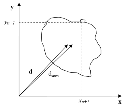
Figure 5: Cell gaining one pixel denotes a distance from the origin of a fixed frame of reference to the center of mass of a cell before the cell gains a new pixel. \(d_{new}\) denotes the same distance but after the cell gains a new pixel
Now, using the parallel axis theorem, we can write an expression for the moment of inertia after the cell gains one pixel:
where, as before, \(I_{xx}^{new}\) denotes the moment of inertia of a cell with a new pixel with
respect to x axis passing through the center of mass, \(I_{x'x'}^{new}\) is a moment of
inertia with respect to an axis parallel to the x axis that passes through the
center of mass, \(d_{new}\) is the distance between the axes, and
\(V+1\) is the volume of the cell after it gained one pixel. Now, let us
rewrite the above equation by adding and subtracting the \(Vd^2\) term:
Therefore, we have found an expression for the moment of inertia passing through the center of mass of the cell with the additional pixel. Note that this expression involves a moment of inertia for the old cell (i.e. the original cell, not the one with extra pixel). When we add a new pixel, we know its coordinates and we can also easily calculate \(d_new\) . Thus, when we need to calculate the moment of inertia for a new cell, instead of performing summation as given in the definition of the inertia tensor, we can use a much simpler expression.
This was a diagonal term of the inertia tensor. What about off-diagonal terms? Let us write an explicit expression for \(I_{xy}\) :
where \(x_{COM}\), \(y_{COM}\) denote x and y center of mass positions of the cell,
\(V\) denotes cell volume. In the above formula, we have used the fact that:
and similarly for the y coordinate.
Now, for the new cell with an additional pixel, we have the following relation:
where we have added and subtracted \(V x_{COM}y_{COM}\) to be able to form \(I_{xy}^{old}- \sum_i^{N} x_i y_i+ V x_{COM}y_{COM}\) on the right hand side of the expression for \(I_{xy}^{new}\) . As was the case for the diagonal element, calculating an off-diagonal of the inertia tensor involves ::math`I_{xy}^{old}` and the center of mass of the cell before and after gaining a new pixel. All those quantities are either known a priori (::math`I_{xy}^{old}`) or can be easily calculated (center of mass position after gaining one pixel).
We have shown how we can calculate the tensor of inertia for a given cell with respect to a coordinate frame with origin at a cell’s center of mass, without evaluating full sums. Such “local” calculations greatly speed up simulations.
Calculating the Shape Constraint of a Cell – the Elongation Term
Related: Calculating Inertia Tensor in CC3D and MomentOfInertia Plugin
- Learning Objectives:
Learn how CC3D leverages inertia tensors to elongate cells
The shape of a single cell immersed in medium and not subject to too drastic surface or surface constraints will be spherical (circular in 2D). However, in certain situations, we may want to use cells that are elongated along one of their body axes. To facilitate, this we can place constraints on the principal lengths of the cell. In 2D, it is sufficient to constrain one of the principal lengths of the cell. However, in 3D, we need to constrain 2 out of 3 principal lengths.
Our first task is to diagonalize the inertia tensor (i.e. find a coordinate frame transformation which brings the inertia tensor to a diagonal form)
Diagonalizing inertia tensor
We will consider here a more difficult 3D case. The 2D case is described in detail in M. Zajac, G.L. Jones, and J.A. Glazier in “Simulating convergent extension by way of anisotropic differential adhesion” Journal of Theoretical Biology 222 (2003) 247–259.
In order to diagonalize the inertia tensor, we need to solve the following eigenvalue equation:
or in full form
The eigenvalue equation will be in the form of 3rd order polynomial. The roots of it are guaranteed to be real. The polynomial itself can be found either by explicit derivation, using symbolic calculation, or simply in Wikipedia ( http://en.wikipedia.org/wiki/Eigenvalue_algorithm )

so in our case, the eigenvalue equation takes the form:
This equation can be solved analytically, again we may use Wikipedia ( http://en.wikipedia.org/wiki/Cubic_function )
Now, the eigenvalues found that way are the principal moments of inertia of a cell. That is they are components of the inertia tensor in a coordinate frame rotated in such a way that off-diagonal elements of the inertia tensor are 0:
In our cell shape constraint, we will want to obtain ellipsoidal cells. Therefore the target tensor of inertia for the cell should be the tensor if inertia for the ellipsoid:
where a, b, c are parameters describing the surface of an ellipsoid:
In other words a, b, c are half lengths of principal axes (they are
analogues of the circle’s radius).
Now we can determine semi axes lengths in terms of principal moments of inertia by inverting the following set of equations:
Once we have calculated semiaxes lengths in terms of moments of inertia, we can plug in actual numbers for moment of inertia (the ones for actual cell) and obtain lengths of semiaxes.
Next, we apply a quadratic constraint on largest (semimajor) and smallest (semiminor axes). This is what the elongation plugin does.
Forward Euler method for solving PDE’s in CompuCell3D.
Note
We present more complete derivations of explicit finite difference scheme for diffusion solver in “Introduction to Hexagonal Lattices in CompuCell3D” (http://www.compucell3d.org/BinDoc/cc3d_binaries/Manuals/HexagonalLattice.pdf).
In CompuCell3D most of the solvers uses explicit schemes (Forward Euler method) to obtain PDE solutions. Thus for the diffusion equation we have:
In a discretetized form we may write:
where to save space we used shorthand notation:
and similarly for other coordinates.
After rearranging terms we get the following expression:
where the sum over index \(i\) goes over neighbors of point \((x,y,z)\) and the neighbors will have the following concentrations: \(c(x+\delta x, t)\), \(c(y+\delta y, t)\), \(c(z+\delta z, t)\) .
Calculating center of mass when using periodic boundary conditions.
When you are running calculation with periodic boundary condition you may end up with situation like in the figure below:
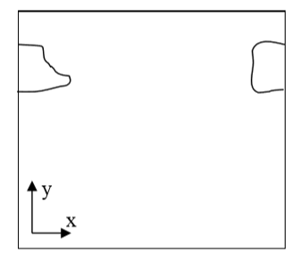
Figure 6 A connected cell in the lattice edge area – periodic boundary conditions are applied
Clearly, what happens is that simply connected cell is wrapped around the lattice edge so part of it is in the region of high values of x coordinate and the other is in the region where x coordinates have low values. Consequently, a naïve calculation of center of mass position according to:
or in vector form:
would result in being somewhere in the middle of the lattice and obviously outside the cell. A better procedure could be as follows:
Before calculating center of mass when new pixel is added or lost we “shift” a cell and new pixel (gained or lost )to the middle of the lattice do calculations “in the middle of the lattice” and shift back. Now if after shifting back it turns out that center of mass of a cell lies outside lattice position it in the center of mass by applygin a shift equal to the length of the lattice and whose direction should be such that the center of mass of the cell ends up inside the lattice (there is only one such shift and it might be be equal to zero vector).
This is how we do it using mathematical formulas:
First we define shift vector \(\vec{s}\) as a vector difference between vector pointing to center of mass of the cell \(\vec{r}_{COM}\) and vector pointing to (approximately) the middle of the lattice \(\vec{c}\).
Next we shift cell to the middle of the lattice using :
where \(\vec{r'}_{COM}\) denotes center of mass position of a cell after shifting but before adding or subtracting a pixel.
Next we take into account the new pixel (either gained or lost) and calculate center of mass position (for the shifted cell):
Above we have assumed that we are adding one pixel.
Now all that we need to do is to shift back \(\vec{r'}_{COM}^{new}\) by same vector \(\vec{s}\) that brought cell to (approximately) center of the lattice:
We are almost done. We still have to check if \(\vec{r'}_{COM}^{new}\) is inside the lattice. If this is not the case we need to shift it back to the lattice but now we are allowed to use only a vector \(\vec{P}\) whose components are multiples of lattice dimensions (and we can safely restrict to +1 and -1 multiples of the lattice dimensions) . For example we may have:
where \(\vec{x}_{max}\), \(\vec{y}_{max}\), \(\vec{z}_{max}\) are dimensions of the lattice.
There is no cheating here. In the lattice with periodic boundary conditions you are allowed to shift point coordinates a vector whose components are multiples of lattice dimensions.
All we need to do is to examine new center of mass position and form suitable vector \(\vec{P}\).
Dividing Clusters (aka compartmental cells)
Related: Compartmentalized Cells, ContactInternal Plugin, and related XML
In compartmental models, a single cell is actually composed of several compartments.
Each compartment is somewhat like an individual cell in that its behaviors
can be specified independently, yet all the compartments can be treated as a single entity called a “cluster.”
A cluster is a collection of compartment cells with the same clusterId. If you use “simple” (non-compartmentalized) cells, then you can check that each such cell has a distinct id and clusterId.
An example simulation can be found in CompuCellPythonTutorial/clusterMitosis.
Let’s look at how we can divide “compact,” that is, “blob-shaped,” clusters.
from cc3d.core.PySteppables import *


class MitosisSteppableClusters(MitosisSteppableClustersBase):

    def __init__(self, frequency=1):
        MitosisSteppableClustersBase.__init__(self, frequency)

    def step(self, mcs):

        for cell in self.cell_list:
            cluster_cell_list = self.get_cluster_cells(cell.clusterId)
            print("DISPLAYING CELL IDS OF CLUSTER ", cell.clusterId, "CELL. ID=", cell.id)
            for cell_local in cluster_cell_list:
                print("CLUSTER CELL ID=", cell_local.id, " type=", cell_local.type)

        mitosis_cluster_id_list = []
        for compartment_list in self.clusterList:
            # print( "cluster has size=",compartment_list.size())
            cluster_id = 0
            cluster_volume = 0
            for cell in CompartmentList(compartment_list):
                cluster_volume += cell.volume
                cluster_id = cell.clusterId

            # condition under which cluster mitosis takes place
            if cluster_volume > 250:
                # instead of doing mitosis right away we store ids for clusters which should be divide.
                # This avoids modifying cluster list while we iterate through it
                mitosis_cluster_id_list.append(cluster_id)

        for cluster_id in mitosis_cluster_id_list:

            self.divide_cluster_random_orientation(cluster_id)

            # # other valid options - to change mitosis mode leave one of the below lines uncommented
            # self.divide_cluster_orientation_vector_based(cluster_id, 1, 0, 0)
            # self.divide_cluster_along_major_axis(cluster_id)
            # self.divide_cluster_along_minor_axis(cluster_id)

    def update_attributes(self):
        # compartments in the parent and child clusters are
        # listed in the same order so attribute changes require simple iteration through compartment list
        compartment_list_parent = self.get_cluster_cells(self.parent_cell.clusterId)

        for i in range(len(compartment_list_parent)):
            compartment_list_parent[i].targetVolume /= 2.0
        self.clone_parent_cluster_2_child_cluster()
The steppable is quite similar to the mitosis steppable which works for
non-compartmental cells. This time, after mitosis happens, you
have to reassign properties of children compartments and of parent
compartments which usually means iterating over a list of compartments.
Conveniently, this iteration is quite simple, and SteppableBasePy class
has a convenience function called get_cluster_cells which returns a list of cells
belonging to a cluster with a given clusterId:
compartment_list_parent = self.get_cluster_cells(self.parent_cell.clusterId)
The call above returns a list of cells in a cluster with clusterId
specified by self.parent_cell.clusterId. In the subsequent for-loop, we
iterate over a list of cells in the parent cluster and assign appropriate
values of volume constraint parameters. Notice that
compartment_list_parent is indexable (ie. we can access directly any
element of the list provided our index is not out of bounds).
for i in range(len(compartment_list_parent)):
    compartment_list_parent[i].targetVolume /= 2.0
Notice that nowhere in the update attribute function we have modified cell types. This is because, by default, the cluster mitosis module assigns cell types to all the cells of the child cluster and it does it in such a way that the child cell looks like a quasi-clone of the parent cell.
The next call in the update_attributes function is
self.clone_parent_cluster_2_child_cluster(). This copies all the attributes
of the cells in the parent cluster to the corresponding cells in the
child cluster. If you would like to copy attributes from parent to child
cell skipping select ones you may use the following code:
compartment_list_parent = self.get_cluster_cells(self.parent_cell.clusterId)

compartment_lis_child = self.get_cluster_cells(self.child_cell.clusterId)

self.clone_cluster_attributes(source_cell_cluster=compartment_list_parent,
                            target_cell_cluster=compartment_list_child,
                            no_clone_key_dict_list=['ATTR_NAME_1', 'ATTR_NAME_2'])
where clone_cluster_attributes function allows specification of this
attributes are not to be copied (in our case cell.dict members
ATTR_NAME_1 and ATTR_NAME_2 will not be copied).
Finally, if you prefer manually setting the parent and child cells, you would use the following code:
class MitosisSteppableClusters(MitosisSteppableClustersBase):

    def __init__(self, frequency=1):
        MitosisSteppableClustersBase.__init__(self, frequency)

    def step(self, mcs):

        for cell in self.cell_list:
            cluster_cell_list = self.get_cluster_cells(cell.clusterId)
            print("DISPLAYING CELL IDS OF CLUSTER ", cell.clusterId, "CELL. ID=", cell.id)
            for cell_local in cluster_cell_list:
                print("CLUSTER CELL ID=", cell_local.id, " type=", cell_local.type)

        mitosis_cluster_id_list = []
        for compartment_list in self.clusterList:
            # print( "cluster has size=",compartment_list.size())
            cluster_id = 0
            cluster_volume = 0
            for cell in CompartmentList(compartment_list):
                cluster_volume += cell.volume
                cluster_id = cell.clusterId

            # condition under which cluster mitosis takes place
            if cluster_volume > 250:
                # instead of doing mitosis right away we store ids for clusters which should be divide.
                # This avoids modifying cluster list while we iterate through it
                mitosis_cluster_id_list.append(cluster_id)

        for cluster_id in mitosis_cluster_id_list:

            self.divide_cluster_random_orientation(cluster_id)

            # # other valid options - to change mitosis mode leave one of the below lines uncommented
            # self.divide_cluster_orientation_vector_based(cluster_id, 1, 0, 0)
            # self.divide_cluster_along_major_axis(cluster_id)
            # self.divide_cluster_along_minor_axis(cluster_id)

    def updateAttributes(self):

        parent_cell = self.mitosisSteppable.parentCell
        child_cell = self.mitosisSteppable.childCell

        compartment_list_child = self.get_cluster_cells(child_ell.clusterId)
        compartment_list_parent = self.get_cluster_cells(parent_cell.clusterId)

        for i in range(len(compartment_list_child)):
            compartment_list_parent[i].targetVolume /= 2.0

            compartment_list_child[i].targetVolume = compartment_list_parent[i].targetVolume
            compartment_list_child[i].lambdaVolume = compartment_list_parent[i].lambdaVolume
A Python helper for mitosis is available from Twedit++’s code snippets:
CC3D Python->Mitosis.
While dividing non-clustered cells is straightforward, doing the same for clustered cells is more challenging. To divide non-clustered cells using the directional mitosis algorithm, we construct a line or a plane passing through the center of mass of a cell and pixels of the cell on one side of the line/plane end up in the child cell and the rest stays in the parent cell. Be sure to use the PixelTracker plugin with mitosis to enable this pixel manipulation. The orientation of the line/plane can be either specified by the user, or we can use CC3D’s built-in feature to calculate the orientation of the principal axes and divide either along the minor or major axis.
With compartmental cells, things get more complicated because: 1) Compartmental cells are composed of many subcells. 2) There can be different topologies of clusters. Some clusters may look “snake-like” and some might be compactly packed blobs of subcells. The algorithm which we implemented in CC3D works in the following way:
We first construct a set of pixels containing every pixel belonging to a cluster cell. You may think of it as a single “regular” cell.
We store volumes of compartments so that we know how big compartments should be after mitosis (they will be half of the original volume)
We calculate the center of mass of the entire cluster and calculate the vector offsets between the center of mass of a cluster and the center of mass of particular compartments as in the figure below:
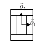
Figure 7. Vectors \(\vec{o}_1\) and \(\vec{o}_2\) show offsets between center of mass of a cluster and center of mass particular compartments.
4) We pick a division line/plane for parent and child cells with offsets between cluster center of mass (after mitosis) and center of masses of clusters. We do it according to the formula:
where \(\vec{p}\) denotes offset after mitosis from the center of mass of child (parent) clusters, \(\vec{o}\) is the orientation vector before mitosis (see picture above), and \(\vec{n}\) is a normalized vector perpendicular to division line/plane. If we try to divide the cluster along a dashed line as in the picture below:
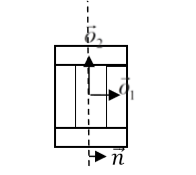
Figure 8. Division of cell along dashed line. Notice the orientation of \(\vec{n}\) . The offsets after the mitosis for child and parent cell will be \(\vec{p}_1=\frac{1}{2}\vec{o}_1\) and \(\vec{p}_2=\vec{o}_2\) as expected because both parent and child cells will retain their heights, but these cells will also become twice as narrow.
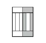
Figure 9.Child and parent cells after mitosis. The parent cell is the one with gray outer compartments.
The formula given above is heuristic. It gives a fairly simple way of assigning pixels of child/parent clusters to cellular compartments. It is not perfect, but the idea is to get the approximate shape of the cell after the mitosis, and, as the simulation runs, the cell shape will readjust based on constraints such as adhesion of focal point plasticity. Before continuing with mitosis, we check if the center of masses of the compartments belong to child/parent clusters. If the center of masses are outside their target pixels, we abandon mitosis and wait for readjustment of the cell shape, at which point the mitosis algorithm will pass this sanity check. For certain “exotic” shapes of cluster shapes, this mitosis algorithm may not work well or at all. In this case, we would have to write a specialized mitosis algorithm.
5) We divide clusters and knowing offsets from the child/parent cluster center of mass we assign pixels to particular compartments. The assignment is based on the distance of the particular pixel to the center of masses of clusters. The pixel is assigned to the compartment if its distance to the center of mass of the compartment is the smallest as compared to distances between centroids of other compartments. If the given compartment has reached its target volume and other compartments are underpopulated, we would assign pixels to other compartments based on the closest distance criterion. Although this method may result in some deviation from perfect 50-50 division of compartment volume, the cells will typically readjust their volume after a few MCS.
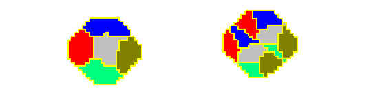
Figure 10. CC3D example of compartmental cell division. See also Demos/CompuCellPythonTutorial/clusterMitosis.
Command line options of CompuCell3D
Although most users run CC3D using Player GUI sometimes it is very convenient to run CC3D using command line options. CC3D allows to invoke Player directly from command line which is convenient because if saves several clicks and if you run many simulations this might be quite convenient.
Remark: On Windows we use .bat extension for run scripts and on Linux/OSX it is .sh. Otherwise all the material in this section applies to all the platforms.
CompuCell3D Player Command Line Options
The command line options for running simulation with the player are as follows:
compucell3d.bat [options]
Options are:
-i <simulation file> - users specify .cc3d simulation file they want to run.
-s <screenshotDescriptionFileName> - name of the file containing
description of screenshots to be taken with the simulation. Usually this
file is prepared using Player by switching to different views, clickin
camera button and saving screenshot description file from the Player
File menu.
-o <customScreenshotDirectoryName> - allows users to specify where
screenshots will be written. Overrides default settings.
--noOutput - instructs CC3D not to store any screenshots. Overrides
Player settings.
--exitWhenDone - instructs CC3D to exit at the end of simulation.
Overrides Player settings.
-h, --help - prints command line usage on the screen
Example command may look like (windows):
compucell3d.bat –i Demos\Models\cellsort\cellsort_2D\cellsort_2d.cc3d --noOutput
or on linux:
compucell3d.sh –i Demos/Models/cellsort/cellsort_2D/cellsort_2d.cc3d --noOutput
and OSX:
compucell3d.command –i Demos/Models/cellsort/cellsort_2D/cellsort_2d.cc3d --noOutput
Running CompuCell3D in a GUI-Less Mode - Command Line Options.
Sometimes when you want to run CC3D on a cluster you will have to use runScript.bat which allows running CC3D simulations without invoking GUI. However, all the screenshots will be still stored.
Remark: current version of this script does not handle properly relative paths so it has to be run from the installation directory of CC3D i.e. you have to cd into this directory prior to runnit runScript.bat. Another solution is to use full paths.
The output of this script is in the form of vtk files which can be subsequently replayed in the Player (and one can take screenshots then). By default all fields present in the simulation are stored in the vtk file. If users want to remove some of the fields from being stored in the vtk format they have to pass this information in the Python script:
CompuCellSetup.doNotOutputField(_fieldName)
Storing entire fields (as opposed to storing screenshots) preserves
exact snapshots of the simulation and allows result postprocessing. In
addition to the vtk files runScript stores lattice description file with
.dml` extension which users open in the Player (File->Open Lattice Description Summary File…)
if they want to reply generated vtk files.
The format of the command (windows):
runScript.bat [options]
linux:
runScript.sh [options]
OSX:
runScript.command [options]
The command line options for runScript.bat are as follows:
-i <simulation file> - users specify .cc3d simulation file they want to run.
-c <outputFileCoreName> - allows users to specify core name for the vtk
files. The default name for vtk files is Step
-o <customVtkDirectoryName> - allows users to specify where vtk files
and the .dml file will be written. Overrides default settings
-f <frequency> or –outputFrequency=<frequency> - allows to specify how
often vtk files are stored to the disk. Those files tend to be quite
large for bigger simulations so storing them every single MCS (default
setting) slows down simulation considerably and also uses a lot of disk
space.
--noOutput - instructs CC3D not to store any output. This option makes
little sense in most cases.
-h, --help - prints command line usage on the screen
Example command may look as follows(windows):
runScript.bat –i Demos\CompuCellPythonTutorial\InfoPrinter\cellsort_2D_info_printer.cc3d –f 10 –o Demos\CompuCellPythonTutorial\InfoPrinter\screenshots –c infoPrinter
linux:
runScript.sh –i Demos/CompuCellPythonTutorial/InfoPrinter/cellsort_2D_info_printer.cc3d –f 10 –o Demos/CompuCellPythonTutorial/InfoPrinter/screenshots –c infoPrinter
osx:
runScript.command –i Demos/CompuCellPythonTutorial/InfoPrinter/cellsort_2D_info_printer.cc3d –f 10 –o Demos/CompuCellPythonTutorial/InfoPrinter/screenshots –c infoPrinter
Managing CompuCell3D simulations (CC3D project files)
Until version 3.6.0 CompuCell3D simulations were stored as a combination
of Python, CC3DML (XML), and PIF files. Starting with version
3.6.0 we introduced new way of managing CC3D simulations by enforcing
that a single CC3D simulation is stored in a folder containing .cc3d
project file describing simulation resources (.cc3d is in fact XML),
such as CC3DML configuration file, Python scripts, PIF files,
Concentration files etc…* and a directory called Simulation where all
the resources reside. The structure of the new-style CC3D simulation is
presented in the diagram below:
->CellsortDemo
CellsortDemo.cc3d
->Simulation
Cellsort.xml
Cellsort.py
CellsortSteppables.py
Cellsort.piff
FGF.txt
Bold fonts denote folders. The benefit of using CC3D project files instead of loosely related files are as follows:
Previously users had to guess which file needs to be open in CC3D – CC3DML or Python. While in a well written simulation one can link the files together in a way that when user opens either one the simulation would work but, nevertheless, such approach was clumsy and unreliable. Starting with
3.6.0users open.cc3dfile and they don’t have to stress out that CompUCell3D will complain with error message.
Warning
The only way to load simulation in CompuCell3D is to use .cc3d project. We no longer
support previous ways of opening simulations
All the files specified in the .cc3d project files are copied to the result output directory along with simulation results (uncles you explicitly specify otherwise). Thus, when you run multiple simulations each one with different parameters, the copies of all CC3DML and Python files are stored eliminating guessing which parameters were associated with particular simulations.
All file paths appearing in the simulation files are relative paths with respect to main simulation folder. This makes simulations portable because all simulation resources are contained withing single folder. In the example above when referring to
Cellsort.pifffile fromCellsort.xmlyou useSimulation/Cellsort.piff. This makes simulations easily exchangeable between collaboratorsNew style of storing CC3D simulations has also another advantage – it makes graphical management of simulation content and simulation generation very easy. As a matetr of fact new component of CC3D suite – Twedit++ - CC3D edition has a graphical tool that allows for easy project file management and it also has new simulation wizard which allows users to build template of CC3D simulation within less than a minute.
Let’s now look in detail at the structure of .cc3d files (we are using XML syntax here):
<Simulation version="3.6.0">
    <XMLScript>Simulation/Cellsort.xml</XMLScript>
    <PythonScript>Simulation/Cellsort.py</PythonScript>
    <Resource Type="Python">Simulation/CellsortSteppables.py</Resource>
   <PIFFile>Simulation/Cellsort.piff</PIFFile>
    <Resource Type="Field" Copy="No">Simulation/FGF.txt</Resource>
</Simulation>
As you can see the structure of the file is quite flat. All that we are
storing there is names of files that are used in the simulation. Two
files have special tags <XMLFile> which specifies name of the CC3DML
file storing “CC3DML portion” of the simulation and <PythonScript> which
specifies main Python script. We have also <PIFFile> tag which is used to
designate PIF files. All other files used in the simulation are referred
to as Resources. For example Python steppable file is a resource of type
“Python” - <Resource Type="Python">Simulation/CellsortSteppables.py</Resource> .
FGF.txt is a resource of type “Field” - <Resource Type="Field" Copy="No">Simulation/FGF.txt</Resource>.
Notice that all the files are specified using paths relative to main simulation directory i.e. w.r.t to the dir in which
.cc3d file resides
As we mentioned before, when you run .cc3d simulation all the files
listed in the project file are copied to result folder. If for
some reason you want to avoid coping of some of the files, simply add
Copy="No" attribute in the tag with file name specification for example”
<PIFFile Copy="No">Simulation/Cellsort.piff</PIFFile>
<Resource Type="Field" Copy="No">Simulation/FGF.txt</Resource>