Plugins Section
In this section we overview CC3DML syntax for all the plugins available in CompuCell3D. Plugins are either energy functions, lattice monitors or store user assigned data that CompuCell3D uses internally to configure simulation before it is run.
CellType Plugin
An example of the plugin that stores user assigned data that is used to
configure simulation before it is run is a CellType Plugin. This plugin
is responsible for defining cell types and storing cell type
information. It is a basic plugin used by virtually every CompuCell
simulation. The syntax is straight forward as can be seen in the example
below:
<Plugin Name="CellType">
  <CellType TypeName="Medium" TypeId="0"/>
  <CellType TypeName="Fluid" TypeId="1"/>
  <CellType TypeName="Wall" TypeId="2" Freeze=""/>
</Plugin>
Here we have defined three cell types that will be present in the
simulation: Medium, Fluid, Wall. Notice that we assign a number – TypeId
– to every cell type. It is strongly recommended that TypeId’s are
consecutive positive integers (e.g. 0,1,2,3...). Medium is traditionally
given TypeId=0 and we recommend that you keep this convention.
Note
Important: Every CC3D simulation must define CellType Plugin and
include at least Medium specification.
Notice that in the example above cell type Wall has extra attribute
Freeze="". This attribute tells CompuCell that cells of frozen type
will not be altered by pixel copies. Freezing certain cell types is a
very useful technique in constructing different geometries for
simulations or for restricting ways in which cells can move.
Global Volume and Surface Constraints
One of the most commonly used energy term in the GGH Hamiltonian is a term that restricts variation of single cell volume. Its simplest form can be coded as show below:
<Plugin Name="Volume">
    <TargetVolume>25</TargetVolume>
    <LambdaVolume>2.0</LambdaVolume>
</Plugin>
By analogy we may define a term which will put similar constraint regarding the surface of the cell:
<Plugin Name="Surface">
    <TargetSurface>20</TargetSurface>
    <LambdaSurface>1.5</LambdaSurface>
</Plugin>
These two plugins inform CompuCell that the Hamiltonian will have two additional terms associated with volume and surface conservation. That is when pixel copy is attempted one cell will increase its volume and another cell will decrease. Thus overall energy of the system changes. Volume constraint essentially ensures that cells maintain the volume which close (this depends on thermal fluctuations) to target volume. The role of surface plugin is analogous to volume, that is to “preserve” surface. Note that surface plugin is commented out in the example above.
The examples shown below apply volume and surface constraints to all cells in the simulation. you can however apply volume and surface constraints to individual cell types or individual cells
Energy terms for volume and surface constraints have the form:
Note
Copying a single pixel may cause surface change in more that two cells – this is especially true in 3D.
VolumeTracker and SurfaceTracker plugins
These two plugins monitor lattice and update volume and surface of the
cells once pixel copy occurs. In most cases users will not call those
plugins directly. They will be called automatically when either Volume
(calls VolumeTracker) or Surface (calls SurfaceTracker) or
CenterOfMass (calls VolumeTracker) plugins are requested. However one
should be aware that in some situations, for example when doing foam
coarsening, where neither Volume nor Surface plugins are called, one may
still want to track changes in surface or volume of cells. In such
situations we explicitly invoke VolumeTracker or Surface Tracker plugin
with the following syntax:
<Plugin Name=”VolumeTracker”/>
or
<Plugin Name=”SurfaceTracker”/>
VolumeFlex Plugin
VolumeFlex plugin is more sophisticated version of Volume Plugin. While
Volume Plugin treats all cell types the same i.e. they all have the same
target volume and lambda coefficient, VolumeFlex plugin allows you to
assign different lambda and different target volume to different cell
types. The syntax for this plugin is straightforward and essentially
mimics the example below.
<Plugin Name="Volume">
    <VolumeEnergyParameters CellType="Prestalk" TargetVolume="68" LambdaVolume="15"/>
    <VolumeEnergyParameters CellType="Prespore" TargetVolume="69" LambdaVolume="12"/>
    <VolumeEnergyParameters CellType="Autocycling" TargetVolume="80" LambdaVolume="10"/>
    <VolumeEnergyParameters CellType="Ground" TargetVolume="0" LambdaVolume="0"/>
    <VolumeEnergyParameters CellType="Wall" TargetVolume="0" LambdaVolume="0"/>
</Plugin>
Note
Almost all CompuCell3D modules which have options Flex or
LocalFlex are implemented as a single C++ module and CC3D, based on
CC3DML syntax used, figures out which functionality to load at the run
time. As a result for the reminder of this reference manual we will
stick to the convention that all Flex and LocalFlex modules will be
invoked using core name of the module only.
Notice that in the example above cell types Wall and Ground have target
volume and coefficient lambda set to 0 – very unusual. That’s because in
this particular case those cells are frozen so the parameters specified
for these cells do not matter. In fact it is safe to remove
specifications for these cell types, but just for the illustration
purposes we left them here.
Using VolumeFlex Plugin you can effectively freeze certain cell types.
All you need to do is to put very high lambda coefficient for the cell
type you wish to freeze. You have to be careful though , because if
initial volume of the cell of a given type is different from target
volume for this cell type the cells will either shrink or expand to
match target volume and only after this initial volume adjustment will
they remain frozen provided LambdaVolume is high enough. Since rapid
changes in the cell volume are uncontrolled (e.g. they can destroy many
neighboring cells) you should opt for more gradual changes. In any case,
we do not recommend this way of freezing cells because it is difficult
to use, and also not efficient in terms of speed of simulation run.
SurfaceFlex Plugin
SurfaceFlex plugin is more sophisticated version of Surface Plugin.
Everything that was said with respect to VolumeFlex plugin applies to
SurfaceFlex. For syntax see example below:
<Plugin Name="Surface">
    <SurfaceEnergyParameters CellType="Prestalk" TargetSurface="90" LambdaSurface="0.15"/>
    <SurfaceEnergyParameters CellType="Prespore" TargetSurface="98" LambdaSurface="0.15"/>
    <SurfaceEnergyParameters CellType="Autocycling" TargetSurface="92" LambdaSurface="0.1"/>
    <SurfaceEnergyParameters CellType="Ground" TargetSurface="0" LambdaSurface="0"/>
    <SurfaceEnergyParameters CellType="Wall" TargetSurface="0" LambdaSurface="0"/>
</Plugin>
VolumeLocalFlex Plugin
VolumeLocalFlex Plugin is very similar to Volume plugin. however this time
you specify lambda coefficient and target volume, individually for each cell.
In the course of
simulation you can change this target volume depending on e.g.
concentration of e.g. ``FGF``in the particular cell. This way you can specify
which cells grow faster, which slower based on a state of the
simulation. This plugin requires you to develop a module (plugin or
steppable) which will alter target volume for each cell. You can do it
either in C++ or even better in Python.
Example syntax:
<Plugin Name="Volume"/>
SurfaceLocalFlex Plugin
This plugin is analogous to VolumeLocalFlex but operates on cell
surface.
Example syntax:
<Plugin Name="Surface"/>
NeighborTracker Plugin
This plugin, as its name suggests, tracks neighbors of every cell. In addition it calculates common contact area between cell and its neighbors. We consider a neighbor this cell that has at least one common pixel side with a given cell. This means that cells that touch each other either “by edge” or by “corner” are not considered neighbors. See the drawing below:
5 |
5 |
5 |
4 |
4 |
5 |
5 |
5 |
4 |
4 |
5 |
5 |
4 |
4 |
4 |
1 |
1 |
2 |
2 |
2 |
1 |
1 |
2 |
2 |
2 |
Figure 1. Cells 5,4,1 are considered neighbors as they have non-zero common surface area. Same applies to pair of cells 4 ,2 and to 1 and 2. However, cells 2 and 5 are not neighbors because they touch each other “by corner”. Notice that cell 5 has 8 pixels cell 4 , 7 pixels, cell 1 4 pixels and cell 2 6 pixels.
To include this plugin in your simulation , add the following code to the CC3DML
<Plugin Name="NeighborTracker"/>
This plugin is used as a helper module by other plugins and steppables
e.g. FocalPointPlasticity plugin uses NeighborTracker plugin.
Chemotaxis
Chemotaxis plugin, is used to simulate chemotaxis
of cells. For every pixel copy, this plugin calculates change of energy
associated with pixel move. There are several methods to define a change
in energy due to chemotaxis. By default we define a chemotaxis using the
following formula:
where \(c(x_{source})\) and \(c(x_{destination})\) denote chemical concentration at the pixel-copy-source and pixel-copy-destination pixel, respectively.
The body of the Chemotaxis plugin description contains sections called
ChemicalField. In this section we tell CompuCell3D which module contains
chemical field that we wish to use for chemotaxis. In our case it is
FlexibleDiffusionSolverFE. Next we specify the name of the field - FGF.
Subsequently, we specify lambda for each cell type so that cells of
different type may respond differently to a given chemical. In
particular types not listed will not respond to chemotaxis at all.
Occasionally we may want to use different formula for the chemotaxis
than the one presented above. Current version of CompCell3D supports the
following definitions of change in chemotaxis energy (Saturation and
SaturationLinear respectively ):
or
where s denotes saturation constant. To use first of the above
formulas we set the value of the saturation coefficient:
<Plugin Name="Chemotaxis">
   <ChemicalField Source="FlexibleDiffusionSolverFE" Name="FGF">
        <ChemotaxisByType Type="Amoeba" Lambda="0"/>
        <ChemotaxisByType Type="Bacteria" Lambda="2000000" SaturationCoef="1"/>
   </ChemicalField>
</Plugin>
Notice that this only requires small change in line where you previously specified only lambda.
<ChemotaxisByType Type="Bacteria" Lambda="2000000" SaturationCoef="1"/>
To use second of the above formulas use SaturationLinearCoef instead of
SaturationCoef:
<Plugin Name="Chemotaxis">
   <ChemicalField Source="FlexibleDiffusionSolverFE" Name="FGF">
      <ChemotaxisByType Type="Amoeba" Lambda="0"/>
     <ChemotaxisByType Type="Bacteria" Lambda="2000000" SaturationLinearCoef="1"/>
   </ChemicalField>
</Plugin>
The lambda value specified for each cell type can also be scaled using the
LogScaled formula according to the concentration of the field at the center of mass of the
chemotaxing cell \(c_{CM}\),
The LogScaled formula is commonly used to mitigate excessive forces on cells
in fields that vary over several orders of magnitude, and can be selected
by setting the value of \(s\) with the attribute LogScaledCoef like as follows,
<ChemotaxisByType Type="Amoeba" Lambda="100" LogScaledCoef="1"/>
Sometimes it is desirable to have chemotaxis at the interface
between only certain types of cells and not between other
cell-type-pairs. In such a case we augment ChemotaxisByType element with
the following attribute:
<ChemotaxisByType Type="Amoeba" Lambda="100 "ChemotactTowards="Medium"/>
This will cause that the change in chemotaxis energy will be non-zero
only for those pixel copy attempts that happen between pixels belonging
to Amoeba and Medium.
Note
The term ChemotactTowards means “chemotax at the interface between”
CC3D supports slight modifications of the above formulas in the
Chemotaxis plugin where \(\Delta E\) is non-zero only if the cell located at \(x_{source}\) after
the pixel copy is non-medium. To enable this mode users need to include
<Algorithm="Regular"/>
tag in the body of CC3DML plugin.
Additionally, Chemotaxis plugin can apply the above formulas using the parameters
and formulas of both the cell located at \(x_{source}\) (if any) and the cell located
at \(x_{destination}\) (if any). To enable this mode users need to include
<Algorithm="Reciprocated"/>
Let’s look at the syntax by studying the example usage of the Chemotaxis plugin:
<Plugin Name="Chemotaxis">
   <ChemicalField Source="FlexibleDiffusionSolverFE" Name="FGF">
        <ChemotaxisByType Type="Amoeba" Lambda="300"/>
        <ChemotaxisByType Type="Bacteria" Lambda="200"/>
   </ChemicalField>
</Plugin>
The definitions of chemotaxis presented so far do not allow specification of chemotaxis parameters individually for each cell. To do this we will use Python scripting. We still need to specify in the CC3DML which fields are important from chamotaxis stand point. Only fields listed in the CC3DML will be used to calculate chemotaxis energy:
…

<Plugin Name="CellType">
    <CellType TypeName="Medium" TypeId="0"/>
    <CellType TypeName="Bacterium" TypeId="1" />
    <CellType TypeName="Macrophage" TypeId="2"/>
    <CellType TypeName="Wall" TypeId="3" Freeze=""/>
</Plugin>

…

<Plugin Name="Chemotaxis">
    <ChemicalField Source="FlexibleDiffusionSolverFE" Name="ATTR">
    <ChemotaxisByType Type="Macrophage" Lambda="20"/>
    </ChemicalField>
</Plugin>

…
In the above excerpt from the CC3DML configuration file we see that
cells of type Macrophage will chemotax in response to ATTR gradient.
Using Python scripting we can modify chemotaxis properties of individual cells as follows:
class ChemotaxisSteering(SteppableBasePy):
        def __init__(self, _simulator, _frequency=100):
            SteppableBasePy.__init__(self, _simulator, _frequency)

        def start(self):

            for cell in self.cellList:
                if cell.type == self.cell_type.Macrophage:
                    cd = self.chemotaxisPlugin.addChemotaxisData(cell, "ATTR")
                    cd.setLambda(20.0)
                    cd.assignChemotactTowardsVectorTypes([self.cell_type.Medium, self.cell_type.Bacterium])
                    break

        def step(self, mcs):
            for cell in self.cellList:
                if cell.type == self.cell_type.Macrophage:
                    cd = self.chemotaxisPlugin.getChemotaxisData(cell, "ATTR")
                    if cd:
                        lam = cd.getLambda() - 3
                        cd.setLambda(lam)
                    break
In the start function for first encountered cell of type Macrophage
(type==self.cell_type.Macrophage) we insert ChemotaxisData object (it determines chemotaxing
properties) and initialize λ parameter to 20. We also initialize vector
of cell types towards which Macrophage cell will chemotax (it will
chemotax towards Medium and Bacterium cells). Notice the break statement
inside the if statement, inside the loop. It ensures that only first
encountered Macrophage cell will have chemotaxing properties altered.
In the step function we decrease lambda chemotaxis by 3 units every 100
MCS. In effect we turn a cell from chemotaxing up ATTR gradient to being
chemorepelled.
In the above example we have more than one macrophage but only one of them has altered chemotaxing properties. The other macrophages have chemotaxing properties set in the CC3DML section. CompuCell3D first checks if local definitions of chemotaxis are available (i.e. for individual cells) and if so it uses those. Otherwise it will use definitions from from the CC3DML.
The ChemotaxisData structure has additional functions which allow to set
chemotaxis formula used. For example we may type:
def start(self):
    for cell in self.cellList:
        if cell.type == self.cell_type.Macrophage:
            cd = self.chemotaxisPlugin.addChemotaxisData(cell, "ATTR")
            cd.setLambda(20.0)
            cd.setSaturationCoef(200.0)
            cd.assignChemotactTowardsVectorTypes([self.cell_type.Medium, self.cell_type.Bacterium])
            break
to activate Saturation formula. To activate SaturationLinear formula we
would use:
cd.setSaturationLinearCoef(2.0)
To activate the LogScaled formula for a cell, we would use:
cd.setLogScaledCoef(3.0)
Warning
When you use chemotaxis plugin you have to make sure that fields that you refer to and module that contains this fields are declared in the CC3DML file. Otherwise you will most likely cause either program crash (which is not as bad as it sounds) or unpredicted behavior (much worse scenario, although unlikely as we made sure that in the case of undefined symbols, CompuCell3D exits)
ExternalPotential Plugin
Chemotaxis plugin is used to cause directional cell movement in response
to chemical gradient. Another way to achieve directional movement is to
use ExternalPotential plugin. This plugin is responsible for imposing a
directed pressure (or rather force) on cells. It is used to implement
persistent motion of cells and its applications can be very diverse.
Example usage of this plugin looks as follows:
<Plugin Name="ExternalPotential">
   <Lambda x="-0.5" y="0.0" z="0.0"/>
</Plugin>
Lambda is a vector quantity and determines components of force along
three axes. In this case we apply force along x pointing in the positive
direction.
Note
Positive component of Lambda vector pushes cell in the negative direction and negative component pushes cell in the positive direction
We can also apply external potential to specific cell types:
<Plugin Name="ExternalPotential">
    <ExternalPotentialParameters CellType="Body1" x="-10" y="0" z="0"/>
    <ExternalPotentialParameters CellType="Body2" x="0" y="0" z="0"/>
    <ExternalPotentialParameters CellType="Body3" x="0" y="0" z="0"/>
</Plugin>
Where in ExternalPotentialParameters we specify which cell type is
subject to external potential (Lambda is specified using x , y , z
attributes).
We can also apply external potential to individual cells. In that case, in the CC3DML section we only need to specify:
<Plugin Name="ExternalPotential"/>
and in the Python file we change lambdaVecX, lambdaVecY, lambdaVecZ,
which are properties of cell. For example in Python we could write:
cell.lambdaVecX = -10
Calculations done by ExternalPotential Plugin are by default based on
direction of pixel copy (similarly as in chemotaxis plugin). One can,
however, force CC3D to do calculations based on movement of center of
mass of cell. To use algorithm based on center of mass movement we use
the following CC3DML syntax:
<Plugin Name="ExternalPotential">

    <Algorithm>CenterOfMassBased</Algorithm>

    …

</Plugin>
Note
In the pixel-based algorithm the typical value of
pixel displacement used in calculations is of the order of 1 (pixel)
whereas typical displacement of center of mass of cell due to single
pixel copy is of the order of 1/cell volume (pixels) – ~ 0.1 pixel. This
implies that to achieve compatible behavior of cells when using center
of mass algorithm we need to multiply lambda’s by appropriate factor,
typically of the order of 10.
CenterOfMass Plugin
CenterOfMass plugin monitors changes n the lattice and updates centroids of the
cell:
where i denotes pixels belonging to a given cell. To obtain
coordinates of a center of mass of a given cell we divide centroids by
cell volume:
This plugin is aware of boundary conditions and centroids are calculated properly regardless which boundary conditions are used. The CC3DML syntax is very simple:
<Plugin Name="CenterOfMass"/>
To access center of mass coordinates from Python we use the following syntax:
print('x-component of COM is:', cell.xCOM)
print ('y-component of COM is:', cell.yCOM)
print ('z-component of COM is:', cell.zCOM)
Warning
Center of mass parameters in Python are read only. Any attempt to modify them will likely mess up the simulation.
Contact Plugin
Contact plugin implements computations of adhesion energy between neighboring cells.
Together with volume constraint contact energy is one of the most commonly used energy terms in the GGH Hamiltonian. In essence it describes how cells “stick” to each other.
The explicit formula for the energy is:
where i and j label two neighboring lattice sites \(\sigma\)’s denote cell
Ids, \(\tau\)’s denote cell types .
In the above formula, we need to differentiate between cell types and
cell Ids. This formula shows that cell types and cell Ids are not the
same. The Contact plugin in the .xml file, defines the energy per unit
area of contact between cells of different types (\(J\left ( \tau_{\sigma(i)},\tau_{\sigma(j)} \right )\)) and the interaction
range NeighborOrder of the contact:
<Plugin Name="Contact">
    <Energy Type1="Foam" Type2="Foam">3</Energy>
    <Energy Type1="Medium" Type2="Medium">0</Energy>
    <Energy Type1="Medium" Type2="Foam">0</Energy>
    <NeighborOrder>2</NeighborOrder>
</Plugin>
In this case, the interaction range is 2, thus only up to second nearest
neighbor pixels of a pixel undergoing a change or closer will be used to calculate
contact energy change. Foam cells have contact energy per unit area of 3
and Foam and Medium as well as Medium and Medium have contact energy of
0 per unit area. For more information about contact energy calculations
see “Introduction to CompuCell3D”
AdhesionFlex Plugin
AdhesionFlex offers a very flexible way to define adhesion between cells. It
allows setting individual adhesivity properties for each cell. Users can
use either CC3DML syntax or Python scripting to initialize adhesion
molecule density for each cell. In addition, Medium can also carry its
own adhesion molecules. We use the following formula to calculate
adhesion energy in AdhesionFlex plugin:
where indexes i, j label pixels, \(- \sum_{m,n}k_{mn}F\left ( N_{m}\left (i \right ), N_{n} \left( j \right ) \right )\)
denotes contact energy between cell types \(\sigma(i)\) and \(\sigma(j)\) and indexes m , n
label adhesion molecules in cells composed of pixels i and j respectively. F
denotes user-defined function of \(N_m\) and \(N_n\).
Although this may look a bit complex, the basic idea is simple: each
cell has certain number of adhesion molecules on its surface. When cells touch
each other the resultant energy is simply a “product of interactions” of
adhesion molecules from one cell with adhesion molecules from another cell. The CC3DML
syntax for this plugin is given below:
<Plugin Name="AdhesionFlex">
    <AdhesionMolecule Molecule="NCad"/>
    <AdhesionMolecule Molecule="NCam"/>
    <AdhesionMolecule Molecule="Int"/>
    <AdhesionMoleculeDensity CellType="Cell1" Molecule="NCad" Density="6.1"/>
    <AdhesionMoleculeDensity CellType="Cell1" Molecule="NCam" Density="4.1"/>
    <AdhesionMoleculeDensity CellType="Cell1" Molecule="Int" Density="8.1"/>
    <AdhesionMoleculeDensity CellType="Medium" Molecule="Int" Density="3.1"/>
    <AdhesionMoleculeDensity CellType="Cell2" Molecule="NCad" Density="2.1"/>
    <AdhesionMoleculeDensity CellType="Cell2" Molecule="NCam" Density="3.1"/>

    <BindingFormula Name="Binary">
        <Formula> min(Molecule1,Molecule2)</Formula>
        <Variables>
            <AdhesionInteractionMatrix>
             <BindingParameter Molecule1="NCad" Molecule2="NCad">-1.0</BindingParameter>
             <BindingParameter Molecule1="NCam" Molecule2="NCam">2.0</BindingParameter>
             <BindingParameter Molecule1="NCad" Molecule2="NCam">-10.0</BindingParameter>
             <BindingParameter Molecule1="Int" Molecule2="Int">-10.0</BindingParameter>
            </AdhesionInteractionMatrix>
        </Variables>
    </BindingFormula>

    <NeighborOrder>2</NeighborOrder>
</Plugin>
\(k_{mn}\) matrix is specified within the AdhesionInteractionMatrix
tag – the elements are listed using BindingParameter tags. The
AdhesionMoleculeDensity tag specifies initial concentration of adhesion
molecules. Even if you are going to modify those from Python you are still required to specify the
names of adhesion molecules and associate them with appropriate cell
types. Failure to do so may result in simulation crash or undefined
behaviors. The user-defined function *F* is specified using Formula tag
where the arguments of the function are called Molecule1 and Molecule2 .
The syntax has to follow syntax of the muParser -
https://beltoforion.de/en/muparser/features.php#idDef1 .
Note
Using more complex formulas with muParser requires special CDATA syntax. Please check muParser for more details.
CompuCell3D example – Demos/AdhesionFlex - demonstrates how to manipulate concentration of adhesion molecules. For example:
self.adhesionFlexPlugin.getAdhesionMoleculeDensity(cell,"NCad")
allows to access adhesion molecule concentration using its name (as
given in the CC3DML above using AdhesionMoleculeDensity tag).
self.adhesionFlexPlugin.getAdhesionMoleculeDensityByIndex(cell,1)
allows to access adhesion molecule concentration using its index in the adhesion molecule density vector. The order of the adhesion molecule densities in the vector is the same as the order in which they were declared in the CC3DML above - AdhesionMoleculeDensity tags.
self.adhesionFlexPlugin.getAdhesionMoleculeDensityVector(cell)
allows access to entire adhesion molecule density vector. Each of these functions has
its corresponding function which operates on
Medium . In this case we do not give cell as first argument:
self.adhesionFlexPlugin.getMediumAdhesionMoleculeDensity('Int')

self.adhesionFlexPlugin.getMediumAdhesionMoleculeDensityByIndex (0)

self.adhesionFlexPlugin.getMediumAdhesionMoleculeDensityVector(cell)
To change the value of the adhesion molecule density we use set functions:
self.adhesionFlexPlugin.setAdhesionMoleculeDensity(cell,'NCad',0.1)

self.adhesionFlexPlugin.setAdhesionMoleculeDensityByIndex(cell,1,1.02)

self.adhesionFlexPlugin.setAdhesionMoleculeDensityVector(cell,[3.4,2.1,12.1])
Notice that in this last function we passed entire Python list as the argument. CC3D will check if the number of entries in this vector is the same as the number of entries in the currently used vector. If so the values from the passed vector will be copied, otherwise they will be ignored.
Note
During mitosis we create new cell (childCell) and the
adhesion molecule vector of this cell will have no components. However
in order for simulation to continue we have to initialize this vector
with number of adhesion molecules appropriate to childCell type. We know that
setAdhesionMoleculeDensityVector is not appropriate for this task so we
have to use:
self.adhesionFlexPlugin.assignNewAdhesionMoleculeDensityVector(cell,[3.4,2.1,12.1])
which will ensure that the content of passed vector is copied entirely into cell’s vector (making size adjustments as necessary).
Note
You have to make sure that the number of newly assigned adhesion molecules is exactly the same as the number of adhesion molecules declared for the cell of this particular type.
All of the get functions has corresponding set function which operates on
Medium:
self.adhesionFlexPlugin.setMediumAdhesionMoleculeDensity("NCam",2.8)

self.adhesionFlexPlugin.setMediumAdhesionMoleculeDensityByIndex(2,16.8)

self.adhesionFlexPlugin.setMediumAdhesionMoleculeDensityVector([1.4,3.1,18.1])

self.adhesionFlexPlugin.assignNewMediumAdhesionMoleculeDensityVector([1.4,3.1,18.1])
Compartmentalized cells. ContactInternal Plugin
Calculating contact energies between compartmentalized cells is analogous to the non-compartmentalized case. The energy expression takes the following form:
where i and j denote pixels , σ(µ,ν) denotes a cell
type of a cell with cluster id µ and cell id ν . In compartmental
cell models a cell is a collection of subcells. Each subcell has a
unique id ν (cell id). In addition to that each subcell will have
additional attribute, a cluster id (µ) that determines to which cluster of
subcells a given subcell belongs. Tthink of a cluster as a cell with
nonhomogenous cytoskeleton. So a cluster corresponds to a biological cell and
subcells (or compartments) represents parts of a cell e.g. a nucleus. The core
idea here is to have different contact
energies between subcells belonging to the same cluster and different
energies for cells belonging to different clusters. Technically subcells
of a cluster are “regular” CompuCell3D cells. By giving them an extra
attribute cluster id ((µ) we can introduce a concept of compartmental cells.
In our convention σ(0,0) denotes medium
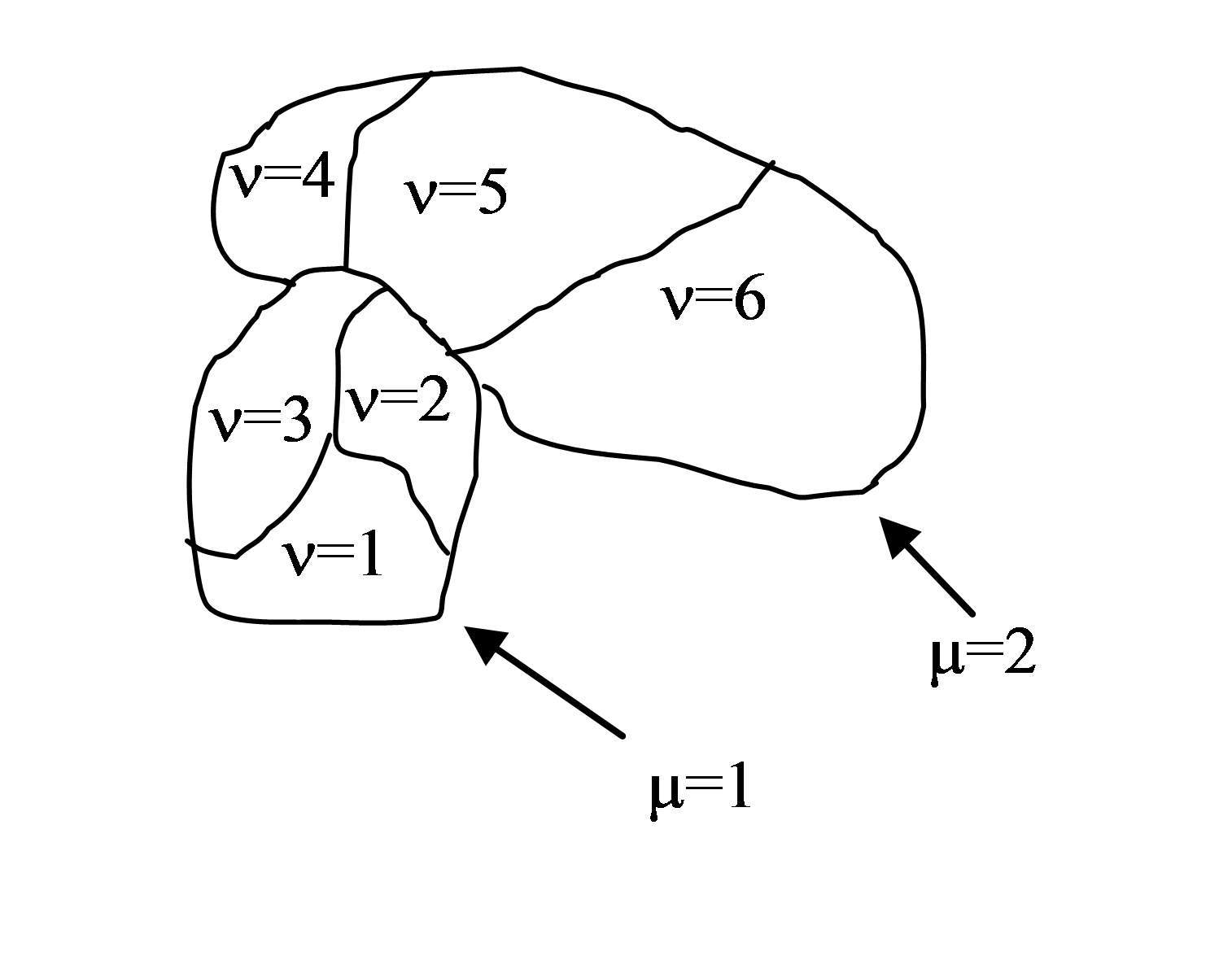
Figure 2. Two compartmentalized cells (cluster id \(\mu=1\) and cluster id \(\mu=2\)). Compartmentalized cell \(\mu=1\) consists of subcells with cell id \(\nu=1,2,3\) and compartmentalized cell \(\mu=2\) consists of subcells with cell id \(\nu=4,5,6\)
Introduction of cluster id and cell id are essential for the definition of \(J\left ( \sigma (\mu_{i},\nu_{i}),\sigma (\mu_{j},\nu_{j}) \right )\)
Indeed:
As we can see from above there are two hierarchies of contact energies –
external and internal. To describe adhesive interactions between
different compartmentalized cells we use two plugins: Contact and
ContactInternal. Contact plugin calculates energy between two cells
belonging to different clusters and ContactInternal calculates energies
between cells belonging to the same cluster. An example syntax is shown
below
<Plugin Name="Contact">

    <Energy Type1="Base" Type2="Base">0</Energy>
    <Energy Type1="Top" Type2="Base">25</Energy>
    <Energy Type1="Center" Type2="Base">30</Energy>
    <Energy Type1="Bottom" Type2="Base">-2</Energy>
    <Energy Type1="Side1" Type2="Base">25</Energy>
    <Energy Type1="Side2" Type2="Base">25</Energy>
    <Energy Type1="Medium" Type2="Base">0</Energy>


    <Energy Type1="Medium" Type2="Medium">0</Energy>
    <Energy Type1="Top" Type2="Medium">30</Energy>
    <Energy Type1="Bottom" Type2="Medium">20</Energy>
    <Energy Type1="Side1" Type2="Medium">30</Energy>
    <Energy Type1="Side2" Type2="Medium">30</Energy>
    <Energy Type1="Center" Type2="Medium">45</Energy>

    <Energy Type1="Top" Type2="Top">2</Energy>
    <Energy Type1="Top" Type2="Bottom">100</Energy>
    <Energy Type1="Top" Type2="Side1">25</Energy>
    <Energy Type1="Top" Type2="Side2">25</Energy>
    <Energy Type1="Top" Type2="Center">35</Energy>

    <Energy Type1="Bottom" Type2="Bottom">10</Energy>
    <Energy Type1="Bottom" Type2="Side1">25</Energy>
    <Energy Type1="Bottom" Type2="Side2">25</Energy>
    <Energy Type1="Bottom" Type2="Center">35</Energy>

    <Energy Type1="Side1" Type2="Side1">25</Energy>
    <Energy Type1="Side1" Type2="Center">25</Energy>
    <Energy Type1="Side2" Type2="Side2">25</Energy>
    <Energy Type1="Side2" Type2="Center">25</Energy>
    <Energy Type1="Side1" Type2="Side2">15</Energy>

    <Energy Type1="Center" Type2="Center">20</Energy>

    <NeighborOrder>2</NeighborOrder>
</Plugin>
and
<Plugin Name="ContactInternal">

    <Energy Type1="Base" Type2="Base">0</Energy>
    <Energy Type1="Base" Type2="Bottom">0</Energy>
    <Energy Type1="Base" Type2="Side1">0</Energy>
    <Energy Type1="Base" Type2="Side2">0</Energy>
    <Energy Type1="Base" Type2="Center">0</Energy>

    <Energy Type1="Top" Type2="Top">4</Energy>
    <Energy Type1="Top" Type2="Bottom">25</Energy>
    <Energy Type1="Top" Type2="Side1">22</Energy>
    <Energy Type1="Top" Type2="Side2">22</Energy>
    <Energy Type1="Top" Type2="Center">15</Energy>

    <Energy Type1="Bottom" Type2="Bottom">4</Energy>
    <Energy Type1="Bottom" Type2="Side1">15</Energy>
    <Energy Type1="Bottom" Type2="Side2">15</Energy>
    <Energy Type1="Bottom" Type2="Center">10</Energy>

    <Energy Type1="Side1" Type2="Side1">11</Energy>
    <Energy Type1="Side2" Type2="Side2">11</Energy>
    <Energy Type1="Side1" Type2="Side2">11</Energy>

    <Energy Type1="Side2" Type2="Center">10</Energy>
    <Energy Type1="Side1" Type2="Center">10</Energy>

    <Energy Type1="Center" Type2="Center">2</Energy>

    <NeighborOrder>2</NeighborOrder>
</Plugin>
Depending whether pixels for which we calculate contact energies belong to the same cluster or not we will use internal or external contact energies respectively.
LengthConstraint Plugin
This plugin imposes elongation constraint on the cell. It “measures” a cell along its “axis of elongation” and ensures that cell length along the elongation axis is close to target length. For detailed description of this algorithm in 2D see Roeland Merks’ paper “Cell elongation is a key to in silico replication of in vitro vasculogenesis and subsequent remodeling” Developmental Biology 289 (2006) 44-54). This plugin is usually used in conjunction with Connectivity Plugin or ConnectivityGlobal Plugin. The syntax is as follows:
<Plugin Name="LengthConstraint">
    <LengthEnergyParameters CellType="Body1" TargetLength="30" LambdaLength="5"/>
</Plugin>
LambdaLength determines the degree of cell length oscillation around
TargetLength parameter. The higher LambdaLength the less freedom a cell
will have to deviate from TargetLength.
In the 3D case we use the following syntax:
<Plugin Name="LengthConstraint">
     <LengthEnergyParameters CellType="Body1" TargetLength="20" MinorTargetLength="5" LambdaLength="100" />
</Plugin>
Notice new attribute called MinorTargetLength. In 3D it is not
sufficient to constrain the “length” of the cell you also need to
constrain “width” of the cell along axis perpendicular to the major axis
of the cell. This “width” is referred to as MinorTargetLength.
The parameters are assigned using Python – see Demos/elongationFlexTest example.
To control length constraint individually for each cell we may use
Python scripting to assign LambdaLength, TartgetLength and in 3D
MinorTargetLength. In Python steppable we typically would write the
following code:
self.lengthConstraintPlugin.setLengthConstraintData(cell,10,20)
which sets length constraint for cell by setting LambdaLength=10 and
TargetLength=20. In 3D we may specify`` MinorTargetLength`` (we set it to 5)
by adding 4th parameter to the above call:
self.lengthConstraintPlugin.setLengthConstraintData(cell,10,20,5)
Note
If we use CC3DML specification of length constraint for certain cell types and in Python we set this constraint individually for a single cell then the local definition of the constraint has priority over definitions for the cell type.
If, in the simulation, we will be setting length constraint for only few individual cells then it is best to manipulate the constraint parameters from the Python script. In this case in the CC3DML we only have to declare that we will use length constraint plugin and we may skip the definition by-type definitions:
<Plugin Name="LengthConstraint"/>
Note
IMPORTANT: When using target length plugins it is important to use connectivity constraint. This constraint will check if a given pixel copy breaks cell connectivity. If it does, the plugin will add large energy penalty (defined by a user) to change of energy effectively prohibiting such pixel copy. In the case of 2D on square lattice checking cell connectivity can be done locally and thus is very fast. In 3D the connectivity algorithm is a bit slower but but its performance is acceptable. Therefore if you need large cell elongations you should always use connectivity in order to prevent cell fragmentation
Connectivity Plugins
The “basic” Connectivity plugin works only in 2D and only on square
lattice and is used to ensure that cells are connected or in other
words to prevent separation of the cell into pieces. The detailed
algorithm for this plugin is described in Roeland Merks’ paper “Cell
elongation is a key to in-silico replication of in vitro
vasculogenesis and subsequent remodeling” Developmental Biology 289
(2006) 44-54). There was one modification of the algorithm as compared
to the paper. Namely, to ensure proper connectivity we had to reject all
pixel copies that resulted in more that two collisions. (see the paper
for detailed explanation what this means).
The syntax of the plugin is straightforward:
<Plugin Name="Connectivity">
    <Penalty>100000</Penalty>
</Plugin>
Note
The value of Penalty is irrelevant because all Connectivity plugins
have a special status. Namely, CC3D will call connectivity plugin to check if the a given pixel copy would
lead to cell fragmentation and if so it will reject the pixel copy without computing
energy-based pixel-copy acceptance function. thus the only thing that matters here is that
penalty parameter is a positive number. Any number
As we mentioned, earlier 2D connectivity algorithm is particularly fast but works only
on Cartesian lattice nad in 2D only. If you are on hex lattice or are working with 3 dimensions
You should use ConnectivityGlobal plugin and there specify so called FastAlgorithm to get
decent performance.
For example (see Demos/PluginDemos/connectivity_global_fast):
<Plugin Name="ConnectivityGlobal">
    <FastAlgorithm/>
    <ConnectivityOn Type="NonCondensing"/>
    <ConnectivityOn Type="Condensing"/>
</Plugin>
will enforce connectivity of cells of type Condensing and NonCondensing and will use “fast algorithm”.
If you want to enforce connectivity for individual cells cells (see Demos/PluginDemos/connectivity_elongation_fast) you would use the following CC3DML code:
<Plugin Name="ConnectivityGlobal">
    <FastAlgorithm/>
</Plugin>
and couple it with the following Python steppable:
class ConnectivityElongationSteppable(SteppableBasePy):
    def __init__(self,_simulator,_frequency=10):
        SteppableBasePy.__init__(self,_simulator,_frequency)

    def start(self):
        for cell in self.cellList:
            if cell.type==1:
                cell.connectivityOn = True

            elif cell.type==2:
                cell.connectivityOn = True
Below we describe a slower version of ConnectivityGlobal plugin that is still supported but has much slower performance and for that reason we encourage you to try faster implementation described above
Note
DEPRECATED
A more general type of connectivity constraint is implemented in
ConnectivityGlobalplugin. In this case we calculate volume of a cell using breadth first search algorithm and compare it with actual volume of the cell. If they agree we conclude that cell connectivity is preserved. This plugin works both in 2D and 3D and on either type of lattice. However, the computational cost of running such algorithm can be quite high so it is best to limit this plugin to cell types for which connectivity of cell is really essential:<Plugin Name="ConnectivityGlobal"> <Penalty Type="Body1">1000000000</Penalty> </Plugin>As we mentioned before the actual value of
Penaltyparameter does not matter as long it is a positive numberIn certain types of simulation it may happen that at some point cells change cell types. If a cell that was not subject to connectivity constraint, changes type to the cell that is constrained by global connectivity and this cell is fragmented before type change this situation normally would result in simulation freeze. However, CompuCell3D, first before applying constraint it will check if the cell is fragmented. If it is, there is no constraint. Global connectivity constraint is only applied when cell is non-fragmented.
Quite often in the simulation we don’t need to impose connectivity constraint on all cells or on all cells of given type. Usually only select cell types or select cells are elongated and therefore need connectivity constraint. In such a case we simply declare
ConnectivityGlobalwith no further specifications taking place in CC3DML The actual connectivity assignments to particular cells take place in PythonIn CC3DML we only declare:
<Plugin Name="ConnectivityGlobal"/>In Python we manipulate/access connectivity parameters for individual cells using the following syntax:
class ElongationFlexSteppable(SteppableBasePy):
    def __init__(self,_simulator,_frequency=10):
        SteppableBasePy.__init__(self, _simulator, _frequency)
        # self.lengthConstraintPlugin=CompuCell.getLengthConstraintPlugin()


    def start(self):
        pass

    def step(self,mcs):
        for cell in self.cellList:
            if cell.type==1:
                self.lengthConstraintPlugin.setLengthConstraintData(cell,20,20) # cell , lambdaLength, targetLength
                self.connectivityGlobalPlugin.setConnectivityStrength(cell,10000000) #cell, strength

            elif cell.type==2:
                self.lengthConstraintPlugin.setLengthConstraintData(cell,20,30)  # cell , lambdaLength, targetLength
                self.connectivityGlobalPlugin.setConnectivityStrength(cell,10000000) #cell, strength
See also example in Demos/PluginDemos/elongationFlexTest.
If you are in 2D and on Cartesian lattice you may instead use
ConnectivityLocalFlexIn this case
In CC3DML we only declare:
<Plugin Name="ConnectivityLocalFlex"/>and in Python:
self.connectivityLocalFlexPlugin.setConnectivityStrength(cell,20.7)
self.connectivityLocalFlexPlugin.getConnectivityStrength(cell)
Secretion / SecretionLocalFlex Plugin
Secretion “by cell type” can and should be handled by the appropriate PDE solver. To implement secretion in individual cells using Python we can use secretion plugin defined in the CC3DML as:
<Plugin Name="Secretion"/>
or as:
<Plugin Name="SecretionLocalFlex"/>
The inclusion of the above code in the CC3DML will allow users to implement secretion for individual cells from Python.
Note
Secretion for individual cells invoked via Python will be called only once per MCS.
Warning
Secretion plugin can be used to implement secretion by
cell type however we strongly advise against doing so. Defining
secretion by cell type in the Secretion plugin will lead to performance
degradation on multi-core machines. Please see section below for more
information if you are still interested in using secretion by cell-type
inside Secretion plugin
Typical use of secretion from Python is demonstrated best in the example below:
class SecretionSteppable(SecretionBasePy):
    def __init__(self, _simulator, _frequency=1):
        SecretionBasePy.__init__(self, _simulator, _frequency)

    def step(self, mcs):
        attrSecretor = self.getFieldSecretor("ATTR")
        for cell in self.cellList:
            if cell.type == 3:
                attrSecretor.secreteInsideCell(cell, 300)
                attrSecretor.secreteInsideCellAtBoundary(cell, 300)
                attrSecretor.secreteOutsideCellAtBoundary(cell, 500)
                attrSecretor.secreteInsideCellAtCOM(cell, 300)
            elif cell.type == 2:
                attrSecretor.secreteInsideCellConstantConcentration(cell, 300)
Note
Instead of using SteppableBasePy class we are using
SecretionBasePy class. The reason for this is that in order for
secretion plugin with secretion modes accessible from Python to behave
exactly as previous versions of PDE solvers (where secretion was done
first followed by the “diffusion” step) we have to ensure that secretion
steppable implemented in Python is called before each Monte Carlo
Step, which implies that it will be also called before “diffusing”
function of the PDE solvers. SecretionBasePy sets extra flag which
ensures that steppable which inherits from SecretionBasePy is called
before MCS (and before all “regular” Python steppables).
There is no magic to SecretionBasePy - if you still want to use
SteppableBasePy as a base class for secretion do so, but remember that you need to set flag:
self.runBeforeMCS=1
to ensure that your new steppable will run before each MCS. See example
below for alternative implementation of SecretionSteppable using
SteppableBasePy as a base class:
class SecretionSteppable(SteppableBasePy):
    def __init__(self,_simulator,_frequency=1):
        SteppableBasePy.__init__(self,_simulator, _frequency)
        self.runBeforeMCS=1
    def step(self,mcs):
        attrSecretor=self.getFieldSecretor("ATTR")
        for cell in self.cellList:
            if cell.type==3:
                attrSecretor.secreteInsideCell(cell,300)
                attrSecretor.secreteInsideCellAtBoundary(cell,300)
                attrSecretor.secreteOutsideCellAtBoundary(cell,500)
                attrSecretor.secreteOutsideCellAtBoundaryOnContactwith(cell,500,[2,3])
                attrSecretor.secreteInsideCellAtCOM(cell,300)
                attrSecretor.uptakeInsideCellAtCOM(cell,300,0.2)
            elif cell.type==2:
                attrSecretor.secreteInsideCellConstantConcentration(cell,300)
The secretion of individual cells is handled through FieldSecretor
objects. FieldSecretor concept is quite convenient because the amount
of Python coding is quite small. To secrete chemical (this is now done
for individual cell) we first create field secretor object:
attrSecretor = self.getFieldSecretor("ATTR")
which allows us to secrete into field called ATTR.
Then we pick a cell and using field secretor we simulate secretion of
chemical ATTR by a cell:
attrSecretor.secreteInsideCell(cell,300)
Currently we support 7 secretion modes for individual cells:
secreteInsideCell– this is equivalent to secretion in every pixel belonging to a cellsecreteInsideCellConstantConcentration– this is equivalent to secretion in every pixel belonging to a cell and setting concentration to fixed, constant levelsecreteInsideCellAtBoundary– secretion takes place in the pixels belonging to the cell boundarysecreteInsideCellAtBoundaryOnContactWith- secretion takes place in the pixels belonging to the cell boundary that touches any of the cells listed as the last argument of the function callsecreteOutsideCellAtBoundary– secretion takes place in pixels which are outside the cell but in contact with cell boundary pixelssecreteOutsideCellAtBoundaryOnContactWith- secretion takes place in pixels which are outside the cell but in contact with cell boundary pixels and in contact with cells listed the last argument of the function callsecreteInsideCellAtCOM– secretion at the center of mass of the cell
and 6 uptake modes:
uptakeInsideCell– this is equivalent to uptake in every pixel belonging to a celluptakeInsideCellAtBoundary– uptake takes place in the pixels belonging to the cell boundaryuptakeInsideCellAtBoundaryOnContactWith- uptake takes place in the pixels belonging to the cell boundary that touches any of the cells listed as the last argument of the function calluptakeOutsideCellAtBoundary– uptake takes place in pixels which are outside the cell but in contact with cell boundary pixelsuptakeOutsideCellAtBoundaryOnContactWith- uptake takes place in pixels which are outside the cell but in contact with cell boundary pixels and in contact with cells listed the last argument of the function calluptakeInsideCellAtCOM– uptake at the center of mass of the cell
Secretion functions use the following syntax:
secrete*(cell,amount,list_of_cell_types)
Note
The list_of_cell_types is used only for function which
implement such functionality i.e. secreteInsideCellAtBoundaryOnContactWith and
secreteOutsideCellAtBoundaryOnContactWith
Uptake functions use the following syntax:
uptake*(cell,max_amount,relative_uptake,list_of_cell_types)
Note
The list_of_cell_types is used only for function which
implement such functionality i.e. uptakeInsideCellAtBoundaryOnContactWith and
uptakeOutsideCellAtBoundaryOnContactWith
Note
Important: The uptake works as follows: when available concentration
is greater than max_amount, then max_amount is subtracted from
current_concentration, otherwise we subtract
relative_uptake*current_concentration.
As you may infer from above, the modes 1-5 require tracking of pixels belonging to cell and pixels belonging to cell boundary. If you are not using those secretion modes you may disable pixel tracking by including:
<DisablePixelTracker/>
or
<DisableBoundaryPixelTracker/>
as shown in the example below:
<Plugin Name="Secretion">

    <DisablePixelTracker/>
    <DisableBoundaryPixelTracker/>

    <Field Name="ATTR" ExtraTimesPerMC=”2”>
        <Secretion Type="Bacterium">200</Secretion>
        <SecretionOnContact Type="Medium" SecreteOnContactWith="B">300</SecretionOnContact>
        <ConstantConcentration Type="Bacterium">500</ConstantConcentration>
    </Field>
</Plugin>
Note
Make sure that fields into which you will be secreting
chemicals exist. They are usually fields defined in PDE solvers. When
using secretion plugin you do not need to specify SecretionData section
for the PDE solvers.
When implementing e.g. secretion inside cell when the cell is in contact with other cell we use neighbor tracker and a short script in the spirit of the below snippet:
for cell in self.cellList:
    attrSecretor = self.getFieldSecretor("ATTR")
    for neighbor, commonSurfaceArea in self.getCellNeighborDataList(cell):
        if neighbor.type in [self.WALL]:
            attrSecretor.secreteInsideCell(cell, 300)
Secretion Plugin (legacy version)
Warning
While we still support Secretion plugin as described
in this section we observed performance degradation when when declaring
<Field> elements inside the plugin. To resolve this issue we encourage
users to implement secretion “by cell type” in the PDE solver and keep
using secretion plugin to implement secretion on a per-cell basis using
Python scripting.
Note
In version 3.6.2 Secretion plugin should not be used with
DiffusionSolverFE or any of the GPU-based solvers.
In earlier version os of CC3D secretion was part of PDE solvers. We
still support this mode of model description however, starting in 3.5.0
we developed separate plugin which handles secretion only. Via secretion
plugin we can simulate cellular secretion of various chemicals. The
secretion plugin allows users to specify various secretion modes in the
CC3DML file – CC3DML syntax is practically identical to the
SecretionData syntax of PDE solvers. In addition to this Secretion
plugin allows users to manipulate secretion properties of individual
cells from Python level. To account for possibility of PDE solver being
called multiple times during each MCS, the Secretion plugin can be
called multiple times in each MCS as well. We leave it up to user the
rescaling of secretion constants when using multiple secretion calls in
each MCS.
Note
Secretion for individual cells invoked via Python will be called only once per MCS.
Typical CC3DML syntax for Secretion plugin is presented below:
<Plugin Name="Secretion">
    <Field Name="ATTR" ExtraTimesPerMC=”2”>
        <Secretion Type="Bacterium">200</Secretion>
        <SecretionOnContact Type="Medium" SecreteOnContactWith="B">300</SecretionOnContact>
        <ConstantConcentration Type="Bacterium">500</ConstantConcentration>
    </Field>
</Plugin>
By default ExtraTimesPerMC is set to 0 - meaning no extra calls to
Secretion plugin per MCS.
Typical use of secretion from Python is demonstrated best in the example below:
class SecretionSteppable(SecretionBasePy):
    def __init__(self, _simulator, _frequency=1):
        SecretionBasePy.__init__(self, _simulator, _frequency)

    def step(self, mcs):
        attrSecretor = self.getFieldSecretor("ATTR")
        for cell in self.cellList:
            if cell.type == 3:
                attrSecretor.secreteInsideCell(cell, 300)
                attrSecretor.secreteInsideCellAtBoundary(cell, 300)
                attrSecretor.secreteOutsideCellAtBoundary(cell, 500)
                attrSecretor.secreteInsideCellAtCOM(cell, 300)
PDESolverCaller Plugin
Warning
In most cases you can specify extra calls to PDE solvers in the solver itself. Thus this plugin is being deprecated. We mention it here for backward compatibility reasons as some of the older CC3D simulations may still be using this plugin.
PDE solvers in CompuCell3D are implemented as steppables . This means
that by default they are called every MCS. In many cases this is
insufficient. For example if diffusion constant is large, then explicit
finite difference method will become unstable and the numerical solution
will have no sense. To fix this problem one could call PDE solver many
times during single MCS. This is precisely the task taken care of by
PDESolverCaller plugin. The syntax is straightforward:
<Plugin Name="PDESolverCaller">
    <CallPDE PDESolverName="FlexibleDiffusionSolverFE"ExtraTimesPerMC="8"/>
</Plugin>
All you need to do is to give the name of the steppable that implements
a given PDE solver and pass let CompCell3D know how many extra times per
MCS this solver is to be called (here FlexibleDiffusionSolverFE was 8
extra times per MCS).
FocalPointPlasticity Plugin
FocalPointPlasticity puts constraints on the
distance between cells’ center of masses. A key feature of this plugin is that
the list of “focal point plasticity neighbors” can change as the
simulation evolves and user has to specifies the maximum number of “focal point
plasticity neighbors” a given cell can have. Let’s look at relatively
simple CC3DML syntax of FocalPointPlasticityPlugin (see
Demos/PluginDemos/FocalPointPlasticity/FocalPointPlasticity example and we will show more complex
examples later):
<Plugin Name="FocalPointPlasticity">
   <Parameters Type1="Condensing" Type2="NonCondensing">
      <Lambda>10.0</Lambda>
      <ActivationEnergy>-50.0</ActivationEnergy>
      <TargetDistance>7</TargetDistance>
      <MaxDistance>20.0</MaxDistance>
      <MaxNumberOfJunctions>2</MaxNumberOfJunctions>
   </Parameters>

   <Parameters Type1="Condensing" Type2="Condensing">
      <Lambda>10.0</Lambda>
      <ActivationEnergy>-50.0</ActivationEnergy>
      <TargetDistance>7</TargetDistance>
      <MaxDistance>20.0</MaxDistance>
      <MaxNumberOfJunctions>2</MaxNumberOfJunctions>
   </Parameters>
   <NeighborOrder>1</NeighborOrder>
</Plugin>
Parameters section describes properties of links between cells.
MaxNumberOfJunctions, ActivationEnergy, MaxDistance and NeighborOrder
are responsible for establishing connections between cells. CC3D
constantly monitors pixel copies and during pixel copy between two
neighboring cells/subcells it checks if those cells are already
participating in focal point plasticity constraint. If they are not,
CC3D will check if connection can be made (e.g. Condensing cells can
have up to two connections with Condensing cells and up to 2 connections
with NonCondensing cells – see first line of Parameters section and
MaxNumberOfJunctions tag). The NeighborOrder parameter determines the
pixel vicinity of the pixel that is about to be overwritten which CC3D
will scan in search of the new link between cells. NeighborOrder 1
(which is default value if you do not specify this parameter) means that
only nearest pixel neighbors will be visited. The ActivationEnergy
parameter is added to overall energy in order to increase the odds of
pixel copy which would lead to new connection.
Once cells are linked the energy calculation is carried out according to the formula:
where \(l_{ij}\) is a distance between center of masses of cells i and j and \(L_{ij}\) is
a target length corresponding to \(l_{ij}\).
\(\lambda_{ij}\) and \(L_{ij}\) between different cell types are
specified using Lambda and TargetDistance tags. The MaxDistance
determines the distance between cells’ center of masses past which the link
between those cells break. When the link breaks, then in order for the
two cells to reconnect they would need to come in contact again.
However it is usually more likely that there will be other
cells in the vicinity of separated cells so it is more likely to
establish new link than restore broken one.
The above example was one of the simplest examples of use of
FocalPointPlasticity. A more complicated one involves compartmental
cells. In this case each cell has separate “internal” list of links
between cells belonging to the same cluster and another list between
cells belonging to different clusters. The energy contributions from
both lists are summed up and everything that we have said when
discussing example above applies to compartmental cells. Sample syntax
of the FocalPointPlasticity plugin which includes compartmental cells is
shown below. We use InternalParameters tag/section to describe links
between cells of the same cluster (see Demos/PluginDemos/FocalPointPlasticity/FocalPointPlasticityCompartments
example):
<Plugin Name="FocalPointPlasticity">

    <Parameters Type1="Top" Type2="Top">
       <Lambda>10.0</Lambda>
       <ActivationEnergy>-50.0</ActivationEnergy>
       <TargetDistance>7</TargetDistance>
       <MaxDistance>20.0</MaxDistance>
       <MaxNumberOfJunctions NeighborOrder="1">1</MaxNumberOfJunctions>
    </Parameters>

    <Parameters Type1="Bottom" Type2="Bottom">
       <Lambda>10.0</Lambda>
       <ActivationEnergy>-50.0</ActivationEnergy>
       <TargetDistance>7</TargetDistance>
       <MaxDistance>20.0</MaxDistance>
       <MaxNumberOfJunctions NeighborOrder="1">1</MaxNumberOfJunctions>
    </Parameters>

    <InternalParameters Type1="Top" Type2="Center">
       <Lambda>10.0</Lambda>
       <ActivationEnergy>-50.0</ActivationEnergy>
       <TargetDistance>7</TargetDistance>
       <MaxDistance>20.0</MaxDistance>
       <MaxNumberOfJunctions>1</MaxNumberOfJunctions>
    </InternalParameters>

    <InternalParameters Type1="Bottom" Type2="Center">
       <Lambda>10.0</Lambda>
       <ActivationEnergy>-50.0</ActivationEnergy>
       <TargetDistance>7</TargetDistance>
       <MaxDistance>20.0</MaxDistance>
       <MaxNumberOfJunctions>1</MaxNumberOfJunctions>
    </InternalParameters>

    <NeighborOrder>1</NeighborOrder>

</Plugin>
We can also specify link constituent law and change it to different form that “spring relation”. To do this we use the following syntax inside FocalPointPlasticity CC3DML plugin:
<LinkConstituentLaw>
    <!--The following variables lare defined by default: Lambda,Length,TargetLength-->

    <Variable Name='LambdaExtra' Value='1.0'/>
    <Formula>LambdaExtra*Lambda*(Length-TargetLength)^2</Formula>

</LinkConstituentLaw>
By default CC3D defines 3 variables (Lambda, Length, TargetLength) which
correspond to \(\lambda_{ij}\) , \(l_{ij}\) and \(L_{ij}\) from the formula
above. We can also define extra variables in the CC3DML (e.g.
LambdaExtra). The actual link constituent law obeys muParser syntax
convention. Once link constituent law is defined it is applied to all
focal point plasticity links. The example demonstrating the use of
custom link constituent law can be found in
Demos/PluginDemos/FocalPointPlasticityCustom.
Sometimes it is necessary to modify link parameters individually for
every cell pair. In this case we would manipulate FocalPointPlasticity
links using Python scripting. Example
Demos/PluginDemos/FocalPointPlasticity/FocalPointPlasticityCompartments demonstrates exactly this
situation. You still need to include CC3DML section as the one shown
above for compartmental cells, because we need to tell CC3D how to link
cells. The only notable difference is that in the CC3DML we have to
include <Local/> tag to signal that we will set link parameters (Lambda,
TargetDistance, MaxDistance) individually for each cell pair:
<Plugin Name="FocalPointPlasticity">
    <Local/>
    <Parameters Type1="Top" Type2="Top">
       <Lambda>10.0</Lambda>
       <ActivationEnergy>-50.0</ActivationEnergy>
       <TargetDistance>7</TargetDistance>
       <MaxDistance>20.0</MaxDistance>
       <MaxNumberOfJunctions NeighborOrder="1">1</MaxNumberOfJunctions>
    </Parameters>
   ...
</Plugin>
Python steppable where we manipulate cell-cell focal point plasticity link properties is shown below:
class FocalPointPlasticityCompartmentsParams(SteppablePy):
    def __init__(self, _simulator, _frequency=10):
        SteppablePy.__init__(self, _frequency)
        self.simulator = _simulator
        self.focalPointPlasticityPlugin = CompuCell.getFocalPointPlasticityPlugin()
        self.inventory = self.simulator.getPotts().getCellInventory()
        self.cellList = CellList(self.inventory)

    def step(self, mcs):
        for cell in self.cellList:
            for fppd in InternalFocalPointPlasticityDataList(self.focalPointPlasticityPlugin, cell):
                self.focalPointPlasticityPlugin.setInternalFocalPointPlasticityParameters(cell, fppd.neighborAddress,
                                                                                          0.0, 0.0, 0.0)
The syntax to change focal point plasticity parameters (or as here internal parameters) is as follows:
setFocalPointPlasticityParameters(cell1, cell2, lambda, targetDistance, maxDistance)
setInternalFocalPointPlasticityParameters(cell1, cell2, lambda, targetDistance, maxDistance)
Similarly, to inspect current values of the focal point plasticity parameters we would use the following Python construct:
for cell in self.cellList:
    for fppd in InternalFocalPointPlasticityDataList(self.focalPointPlasticityPlugin, cell):
        print "fppd.neighborId", fppd.neighborAddress.id
        " lambda=", fppd.lambdaDistance
For non-internal parameters we simply use FocalPointPlasticityDataList
instead of InternalFocalPointPlasticityDataList .
Examples Demos/PluginDemos/FocalPointPlasticity… show in relatively simple way how
to use FocalPointPlasticity plugin. Those examples also contain useful
comments.
Note
When using FocalPointPlasticity Plugin from Mitosis module one might
need to break or create focal point plasticity links. To do so
FocalPointPlasticity Plugin provides 4 convenience functions which can
be invoked from the Python level:
deleteFocalPointPlasticityLink(cell1, cell2)

deleteInternalFocalPointPlasticityLink(cell1, cell2)

createFocalPointPlasticityLink(cell1, cell2, lambda , targetDistance, maxDistance)

createInternalFocalPointPlasticityLink(cell1, cell2, lambda , targetDistance, maxDistance)
Working on the Basis of Links
Note
All functionality described in this section is relevant for CC3D versions 4.2.4+.
CC3D performs all link calculations on the basis of link objects. That is,
every link as described so far is an object with properties and functions that, much like CellG
objects, can be created, destroyed and manipulated. As such, CC3DML specification tells CC3D to simulate links
and what types of links should be automatically created, but links can also be individually accessed, manipulated,
created and destroyed in Python. FocalPointPlasticity Plugin always uses the basis of links for link calculations,
and so the <Local/> tag in CC3DML FocalPointPlasticity Plugin specification is no longer necessary.
CC3D describes three types of links
FocalPointPlasticityLink: a link between two cells
FocalPointPlasticityInternalLink: a link between two cells of the same cluster
FocalPointPlasticityAnchor: a link between a cell and a point
FocalPointPlasticityLink objects are automatically created from the CC3DML FocalPointPlasticity Plugin
specification in the tag Parameters,
FocalPointPlasticityInternalLink objects are automatically created from CC3DML specification in the tag
InternalParameters, and FocalPointPlasticityAnchor objects are only created in Python.
CompuCell3D/core/Demos/PluginDemos/FocalPointPlasticityLinks demonstrates basic usage of
FocalPointPlasticityLink, the pattern of which is mostly the same for FocalPointPlasticityInternalLink
and FocalPointPlasticityAnchor except for naming conventions of certain properties, functions and objects.
CC3D adopts the convention that for every link with a cell pair (i.e., FocalPointPlasticityLink and
FocalPointPlasticityInternalLink), one cell is the initiator cell (i.e., the cell that initated the link), and
the other cell is the initiated cell. Using this convention, every link has the following API for manipulating
link properties,
# --------------
# | Properties |
# --------------
# Link length; automatically updated by CC3D
length
# Link tension = 2 * lambda * (distance - target_distance); automatically updated by CC3D
tension
# A general python dictionary
dict
# SBML solvers (as on CellG)
sbml
# -----------
# | Methods |
# -----------
# Given one cell, returns the other cell of a link
getOtherCell(self, _cell: CellG) -> CellG
# Returns True if the cell is the initiator
isInitiator(self, _cell: CellG) -> bool
# Get lambda distance
getLambdaDistance(self) -> float
# Set lambda distance
setLambdaDistance(self, _lm: float) -> None
# Get target distance
getTargetDistance(self) -> float
# Set target distance
setTargetDistance(self, _td: float) -> None
# Get maximum distance
getMaxDistance(self) -> float
# Set maximum distance
setMaxDistance(self, _md: float) -> None
# Get maximum number of junctions
getMaxNumberOfJunctions(self) -> int
# Set maximum number of junctions
setMaxNumberOfJunctions(self, _mnj: int) -> None
# Get activation energy
getActivationEnergy(self) -> float
# Set activation energy
setActivationEnergy(self, _ae: float) -> None
# Get neighbor order
getNeighborOrder(self) -> int
# Set neighbor order
setNeighborOrder(self, _no: int) -> None
# Get initialization step; automatically recorded at instantiation
getInitMCS(self) -> int
So, for example, the value of \(\lambda_{ij}\) for a link can be retrieved with link.getLambdaDistance(),
and can be set with link.setLambdaDistance(lambda_ij) for some float-valued variable lambda_ij. Links
automatically created by CC3D according to CC3DML specification are initialized with properties accordingly.
Additionally, FocalPointPlasticityLink and FocalPointPlasticityInternalLink objects have the property
cellPair, which contains, in order, the initiator and initiated cells of the link, while
each FocalPointPlasticityAnchor has the property cell (i.e., the linked cell) and additional methods related
to its anchor point,
Steppables have built-in method for creating and destroying each type of link,
# Create a link between two cells
new_fpp_link(self, initiator: CellG, initiated: CellG, lambda_distance: float, target_distance: float,
             max_distance: float) -> FocalPointPlasticityLink
# Create an internal link between two cells of a cluster
new_fpp_internal_link(self, initiator: CellG, initiated: CellG, lambda_distance: float,
                      target_distance: float, max_distance: float) -> FocalPointPlasticityInternalLink
# Create an anchor
# Anchor point can be specified by individual components x, y and z, or by Point3D pt
new_fpp_anchor(self, cell: CellG, lambda_distance: float, target_distance: float,
               max_distance: float, x: float = 0.0, y: float = 0.0, z: float = 0.0,
               pt: Point3D = None) -> FocalPointPlasticityAnchor
# Destroy a link type FocalPointPlasticityLink, FocalPointPlasticityInternalLink or FocalPointPlasticityAnchor
delete_fpp_link(self, _link) -> None
# Destroy all links attached to a cell by link type
# links, internal_links and anchors selects which type, or all types if not specified
remove_all_cell_fpp_links(self, _cell: CellG, links: bool = False, internal_links: bool = False,
                          anchors: bool = False) -> None
Steppables also have built-in methods for retrieving information about links in simulation, by cell, and by cell pair. These methods are as follows,
# Get number of links
get_number_of_fpp_links(self) -> int
# Get number of internal links
get_number_of_fpp_internal_links(self) -> int
# Get number of anchors
get_number_of_fpp_anchors(self) -> int
# Get link associated with two cells
get_fpp_link_by_cells(self, cell1: CellG, cell2: CellG) -> FocalPointPlasticityLink
# Get internal link associated with two cells
get_fpp_internal_link_by_cells(self, cell1: CellG, cell2: CellG) -> FocalPointPlasticityInternalLink
# Get anchor assicated with a cell and anchor id
get_fpp_anchor_by_cell_and_id(self, cell: CompuCell.CellG, anchor_id: int) -> FocalPointPlasticityAnchor
# Get list of links by cell
get_fpp_links_by_cell(self, _cell: CellG) -> FPPLinkList
# Get list of internal links by cell
get_fpp_internal_links_by_cell(self, _cell: CellG) -> FPPInternalLinkList
# Get list of anchors by cell
get_fpp_anchors_by_cell(self, _cell: CellG) -> FPPAnchorList
# Get list of cells linked to a cell
get_fpp_linked_cells(self, _cell: CompuCell.CellG) -> mvectorCellGPtr
# Get list of cells internally linked to a cell
get_fpp_internal_linked_cells(self, _cell: CellG) -> mvectorCellGPtr
# Get number of link junctions by type for a cell
get_number_of_fpp_junctions_by_type(self, _cell: CellG, _type: int) -> int
# Get number of internal link junctions by type for a cell
get_number_of_fpp_internal_junctions_by_type(self, _cell: CompuCell.CellG, _type: int) -> int
Curvature Plugin
The Curvature plugin implements energy term for compartmental cells. The mathematics
and mechanics between the plugin have been described in
“A New Mechanism for Collective Migration in Myxococcus xanthus”,
J. Starruß, Th. Bley, L. Søgaard-Andersen and A. Deutsch, Journal of
Statistical Physics, DOI: 10.1007/s10955-007-9298-9, (2007). For a
“long” compartmental cell composed of many subcells (think of a snake-like elongated sequence of compartments)
it imposes a constraint on curvature of cells. The syntax is slightly complex:
<Plugin Name="Curvature">

   <InternalParameters Type1="Top" Type2="Center">
      <Lambda>100.0</Lambda>
      <ActivationEnergy>-50.0</ActivationEnergy>
   </InternalParameters>

   <InternalParameters Type1="Center" Type2="Center">
      <Lambda>100.0</Lambda>
      <ActivationEnergy>-50.0</ActivationEnergy>
   </InternalParameters>

   <InternalParameters Type1="Bottom" Type2="Center">
      <Lambda>100.0</Lambda>
      <ActivationEnergy>-50.0</ActivationEnergy>
   </InternalParameters>

   <InternalTypeSpecificParameters>
      <Parameters TypeName="Top" MaxNumberOfJunctions="1" NeighborOrder="1"/>
      <Parameters TypeName="Center" MaxNumberOfJunctions="2" NeighborOrder="1"/>
      <Parameters TypeName="Bottom" MaxNumberOfJunctions="1" NeighborOrder="1"/>
   </InternalTypeSpecificParameters>

</Plugin>
The InternalTypeSpecificParameter informs Curvature Plugin how many
neighbors a cell of given type will have. In the case of “snake-shaped” cell
the numbers that make sense are 1 and 2. The middle segment will have 2
connections and head and tail segments will have only one connection with neighboring
segments (subcells). The connections are established dynamically. The way
it happens is that during simulation CC3D constantly monitors pixel
copies and during pixel copy between two neighboring cells/subcells it
checks if those cells are already “connected” using curvature
constraint. If they are not, CC3D will check if connection can be made
(e.g. Center cells can have up to two connections and Top and Bottom
only one connection). Usually establishing connections takes place at
the beginning of the simulation and often happens within first Monte
Carlo Step (depending on actual initial configuration, of course, but if
segments touch each other connections are established almost
immediately). The ActivationEnergy parameter is added to overall energy
in order to increase the odds of pixel copy which would lead to new
connection. Lambda tag/parameter determines “the strength” of curvature
constraint. The higher the Lambda the more stiffer cells will be i.e.
they will tend to align along straight line.
BoundaryPixelTracker Plugin
BoundaryPixelTracker plugin keeps a list of boundary pixels for each cell. The
syntax is as follows:
<Plugin Name="BoundaryPixelTracker">
   <NeighborOrder>1</NeighborOrder>
</Plugin>
This plugin is also used by other plugins as a helper module. Examples use of this plugin is found in Demos/PluginDemos/BoundaryPixelTracker_xxx.
GlobalBoundaryPixelTracker Plugin
GlobalBoundaryPixelTracker plugin tracks boundary pixels of all
the cells including Medium. It is used in a Boundary Walker algorithm
where instead of blindly picking pixel copy candidate we pick it from the set of pixels comprising
boundaries of non frozen cells. In situations when lattice is large and
there are not that many cells it makes sense to use BoundaryWalker
algorithm to limit number of pixel picks that would not lead to actual pixel copy.
Note
BoundaryWalkerAlgorithm does not really work with OpenMP
version of CC3D which includes all versions starting with 3.6.0.
Take a look at the following example:
<Potts>
   <Dimensions x="100" y="100" z="1"/>
   <Anneal>10</Anneal>
   <Steps>10000</Steps>
   <Temperature>5</Temperature>
   <Flip2DimRatio>1</Flip2DimRatio>
   <NeighborOrder>2</NeighborOrder>
   <MetropolisAlgorithm>BoundaryWalker</MetropolisAlgorithm>
   <Boundary_x>Periodic</Boundary_x>
 </Potts>

 <Plugin Name="GlobalBoundaryPixelTracker">
    <NeighborOrder>2</NeighborOrder>
 </Plugin>
Here we are using BoundaryWalker algorithm (Potts section) and
subsequently we list GlobalBoundaryTracker plugin where we set neighbor
order to match that in the Potts section. The neighbor order determines
how “thick” the overall boundary of cells will be. The higher this
number the more pixels will belong to the boundary.
PixelTracker Plugin
PixelTracker plugin allows storing list of all pixels belonging to a given cell.
The syntax is as follows:
<Plugin Name="PixelTracker">
   <TrackMedium/>
</Plugin>
This plugin is also used by other modules (e.g. Mitosis) as a helper
module. Simple example can be found in Demos/PluginDemos/PixelTrackerExample.
Beginning with 4.1.2, medium pixels can be optionally tracked using TrackMedium.
This feature is automatically enabled by attaching a Fluctuation Compensator to a
PDE solver.
MomentOfInertia Plugin
MomentOfInertia plugin keeps up-to-date tensor of inertia for every cell. Internally, it uses
parallel axis theorem to calculate most up-to-date tensor of inertia. While, the plugin
can be called directly:
<Plugin Name="MomentOfInertia"/>
most commonly it is called indirectly by other plugins like e.g. LengthConstraint
plugin.
MomentOfInertia plugin gives users access (via Python scripting) to
current lengths of cell’s semiaxes. Examples in Demos/PluginDemos/MomentOfInertia
demonstrate how to get lengths of semiaxes. For example, to get semiaxes lengths for
a given cell, in Python we would type:
axes=self.momentOfInertiaPlugin.getSemiaxes(cell)
axes is a 3-component vector with 0th element being length of
minor axis, 1st – length of median axis (which is set to 0 in
2D) and 2nd element indicating the length of major semiaxis.
Note
Important: Because calculating lengths of semiaxes involves quite a
few of floating point operations it may happen (usually on hexagonal
lattice) that for cells composed of 1, 2, or 3 pixels one moment the
square of one of the semiaxes may end up being slightly negative leading
to NaN (not a number) length. This is due to round-off error and whenever
CC3D detects very small absolute value of square of the length of
semiaxes (10-6) it sets length of this semiaxes to 0.0 regardless
whether the squared value is positive or negative. However, it is a good
practice to test whether the length of semiaxis is sane by adding a simple
if statement as shown below (here we show how to test for a NaN):
if length != length:
    print "length is NaN":
else:
    print "length is a proper floating point number"
ConvergentExtension plugin
Note
This is very specialized plugin which currently is in Tier 2 plugins in terms of support. It attempts to implement energy term described in “Simulating Convergent Extension by Way of Anisotropic Differemtial Adhesion”, Zajac M, Jones GL, and Glazier JA, Journal of Theoretical Biology 222 (2), 2003. However due to certain ambiguities in the plugin description we had difficulties to getting it to work properly.
Note
A better way to implement convergent extension is to follow the simulations described in “Filopodial-Tension Model of Convergent-Extension of Tissues”, Julio M. Belmonte , Maciej H. Swat, James A. Glazier, PLoS Comp Bio https://doi.org/10.1371/journal.pcbi.1004952
ConvergentExtension plugin presented here is a somewhat simplified version of
energy term described Mark Zajac’s paper.
This plugin uses the following syntax:
<Plugin Name="ConvergentExtension">
   <Alpha Type="Condensing" >0.99</Alpha>
   <Alpha Type="NonCondensing" >0.99</Alpha>
   <NeighborOrder>2</NeighborOrder>
</Plugin>
The Alpha tag represents numerical value of α parameter from the paper.